Syllabus
- Linear Algebra basics
- Numpy Essentials
- Linear Regression
- Cost function
- Gradient Descent
- Multivariable Linear Regression
- Logistic Regression
- Theano Basics
- Neural Networks
- Introduction to Keras
- Backpropagation
Linear Algebra Revision
To study advanced machine learning, it is recommended to know a few concepts in Linear Algebra like Matrix calculus, Eigen Decomposition, etc. But for this course, we just need to remember a few matrix operations like matrix addition, multiplication, inversion from high school. Let’s start with how we represent a matrix. A matrix is typically of 2 dimensions, represented by [m,n]. A matrix with just one row or one column is called a vector.
To practice these operations, instead of pen and paper approach, let us run the operations using numpy. Numpy is a python library that lets us create and operate on large matrices efficiently. Open up a terminal to get started.
# remove numpy
sudo apt-get remove python-numpy
# install latest version through pip
sudo pip install numpy -U
# open ipython
ipython
import numpy as np
np.zeros([3,3])
# should give zero matrix of shape [3x3]
np.eye(4)
# should give a [4x4] identity matrix
np.random.random([2,3])
# should give a [2x3] matrix of random numbersAddition
\[A + I = C\\ \begin{bmatrix}1 & 2 & 3\\4 & 5 & 6 \\ 7 & 8 & 9\end{bmatrix} + \begin{bmatrix}1 & 0 & 0\\0 & 1 & 0 \\ 0 & 0 & 1\end{bmatrix} = \begin{bmatrix}2 & 2 & 3\\4 & 6 & 6 \\ 7 & 8 & 10\end{bmatrix}\]# Addition in numpy
a = np.array([[1,2,3],[4,5,6],[7,8,9]])
i = np.eye(3)
a+iSubtraction
\[A - I = D\\ \begin{bmatrix}1 & 2 & 3\\4 & 5 & 6 \\ 7 & 8 & 9\end{bmatrix} - \begin{bmatrix}1 & 0 & 0\\0 & 1 & 0 \\ 0 & 0 & 1\end{bmatrix} = \begin{bmatrix}0 & 2 & 3\\4 & 4 & 6 \\ 7 & 8 & 8\end{bmatrix}\]# Subtraction in numpy
a = np.array([[1,2,3],[4,5,6],[7,8,9]])
i = np.eye(3)
a-iMultiplication
\[A \cdot I = I \cdot A = A\\ \begin{bmatrix}1 & 2 & 3\\4 & 5 & 6 \\ 7 & 8 & 9\end{bmatrix} \cdot \begin{bmatrix}1 & 0 & 0\\0 & 1 & 0 \\ 0 & 0 & 1\end{bmatrix} = \begin{bmatrix}1 & 2 & 3\\4 & 5 & 6 \\ 7 & 8 & 9\end{bmatrix}\\\\ A \cdot B = E\\ \begin{bmatrix}1 & 2 & 3\\4 & 5 & 6 \\ 7 & 8 & 9\end{bmatrix} \cdot \begin{bmatrix}6 & 5 & 7\\2 & 8 & 8 \\ 0 & 3 & 9\end{bmatrix} = \begin{bmatrix}6 & 10 & 21\\8 & 40 & 48 \\ 0 & 24 & 81\end{bmatrix}\\\]# Muliplication with identity
a = np.array([[1,2,3],[4,5,6],[7,8,9]])
i = np.eye(3)
print(np.dot(a,i))
print(np.dot(i,a))
# Multiplication a.b
b = np.array([[6, 5, 7],[2, 8, 8],[0, 3, 9]])
print(np.dot(a,b))More Operations
# Transpose of matrix
x = np.arange(1,10).reshape([3,3])
print(x)
print(x.T)
# Inverse of a matrix
y = np.linalg.inv(x)
print(y)
Numpy Essentials
| Task | Function | Snippet |
|---|---|---|
| Convert a list to numpy array | np.array() | np.array([1,2,3,4]) |
| Create a null vector of size 10 | np.zeros() | np.zeros(10) |
| Create a vector with values ranging from 10 to 49 | np.arange() | np.arange(10,50) |
| Create a 3x3 matrix with values ranging from 0 to 8 | np.reshape() | np.arange(9).reshape(3,3) |
| Create a 3x3 identity matrix | np.eye() | np.eye(3) |
| Create a 3x2x2 array with random values | np.random.random() | np.random.random([3,2,2]) |
| Create a 4x4 array (x) with random integers from 0-99 | np.random.randint() | x = np.random.randint(0,100,[4,4]) |
| Find the index of maximum of x | np.argmax(), np.unravel_index | np.unravel_index(x.argmax(),x.shape) |
| Find the index of minimum of x | np.argmin(), np.unravel_index | np.unravel_index(x.argmin(),x.shape) |
| Find mean of x | np.mean() | x.mean() |
| Find sum of all elements in x | np.sum() | x.sum() |
| Find the datatype of x | np.dtype | x.dtype |
| Set datatype of x as float32 | np.astype() | x.astype(‘float32’) |
Linear Regression
Regression is a statistical method for modeling the relationship between a set of (independent) variables. Linear regression basically assumes a linear model. What is linear model? A model that is linear in parameters but can still use the independent variables in non-linear forms like \(x^{2}\) and \(\log x\).
The model is defined by Hypothesis, which is a function of variables and parameters. \(H = a + bx\)
In the equation above, [a,b] is the set of parameters and x is the independent variable. Our objective in regression, is to find the parameters [a,b]. Usually we are given a table of values of variables(x) and outputs(y) and asked to build a model that approximates the relationship between x and y.
def hyp(x,theta,m):
    return np.dot(theta,x.reshape([2,m]))
Download the whole table from here.
| x | y |
|---|---|
| 6.1101 | 17.592 |
| 5.5277 | 9.1302 |
| 8.5186 | 13.662 |
| 7.0032 | 11.854 |
| 5.8598 | 6.8233 |
| …. | …. |
| 5.8707 | 7.2029 |
| 5.3054 | 1.9869 |
| 8.2934 | 0.14454 |
| 13.394 | 9.0551 |
# read data (x,y) from file
def readDataset(filename='ex1data1.txt'):

    with open(filename) as csvfile:
        reader = csv.reader(csvfile)
        datlist = list(reader)
    # return as numpy array
    return np.array(datlist,dtype='float32')

x,y = readDataset().T
First we define a hypothesis, \(h=a + bx\). Now our objective is to find the best values of a and b that closely fits the relationship between x and y, in other words find a,b such that \(h \approx y\).
Cost Function
The cost or loss or error function calculates the difference between the hypothesis and the actual model (i.e) How wrong are the values of a and b? For linear regression, we define cost function as:
\[L = (1/2m)\sum_{i=1}^{m}(h-y)^2\]By measuring the error in the hypothesis we can adjust the parameters a and b to decrease the error. Now this becomes the core function of regression. We adjust the parameters, check the error, adjust them again and on and on; eventually we get the best set of parameters and hence the best fitting model. We call this iterative process, learning. But how exactly do we adjust the parameters?
def cost(x,y,theta):
    m = y.shape[0]
    h = np.dot(theta,x.reshape([2,m]))
    #print(h.shape,x.shape,y.shape,theta.shape)
    return np.sum(np.square(y-h))/(2.0*m)
Gradient Descent
Gradient Descent is an optimization technique that improves the parameters of the model, step by step. In each iteration, a small step is taken in the direction of the local minima of the cost function. The distance of movement in each step, is called the learning rate. If the learning rate is too small, it takes a long time for the model to converge (to fit the data well) and if it is too big, the model might not converge. The value of learning rate(\(\alpha\)) is thus, crucial to the learning process.
\[a : a - (1/m) \alpha \nabla_{a}\\ b : b - (1/m) \alpha \nabla_{b}\\ \nabla_{a} = \sum_{i=1}^{m} (h_{i} - y_{i})\\ \nabla_{b} = \sum_{i=1}^{m} (h_{i} - y_{i})x_{i}\\\]def gd(x,y,theta,alpha = 0.005,iter=10000):
m = y.shape[0]
for i in range(iter):
h = hyp(x,theta,m)
error = h-y
update = np.dot(x,error)
theta = theta - ( (alpha*update)/m )
print('theta',theta)
print('cost',cost(x,y,theta))Multivariable Linear Regression
What we have seen so far, is Simple Linear Regression, which models the relationsip between two scalar variables. In multivariable linear regression, we will deal with a vector of inputs.
Hypothesis, \(H = \theta^{T} X\\\) where \(X, \theta\) are vectors
X is a vector of [\(x_1, x_2, x_3,...x_n\)] and \(\theta\) is a vector of all the parameters [\(\theta_0, \theta_1,...\theta_n\)].
def hyp(x,theta,m):
    return np.dot(theta,x.reshape([3,m]))
Cost function
\[L = (1/2m)\sum (Y-H)\]def cost(x,y,theta):
m = y.shape[0]
h = np.dot(theta,x.reshape([3,m]))
#print(h.shape,x.shape,y.shape,theta.shape)
return np.sum(np.square(y-h))/(2.0*m)
Gradient Descent
def gd(x,y,theta,alpha = 0.005,iter=1000000):
    m = y.shape[0]

    for i in range(iter):
        h = hyp(x,theta,m)
        error = h-y
        update = np.dot(x,error)
        theta = theta - ( (alpha*update)/m )

    print('theta',theta)
    print('cost',cost(x,y,theta))
Logistic Regression
Logistic Regression is a regression technique where the output variable is categorical (note that the output variable is continuous in the previous cases). Categorical means that the output variable can only take a limited set of values. Take the case of Binary Logistic Regression model where the output is either zero or one [0,1]. Similarly we can build a model such that the output is [0,1,2,3,4,5,6,7,8,9]. Such a model can be used for classification of images of characters [A-Z] or digits [0-9]. The logistic regression model can also be called a classifier.
The hypothesis is defined as
\[h = g(\theta^{T}X)\]where \(g\) is a sigmoid function, which squashes the input \(\theta^{T}X\) into the range (0,1).
def hyp(x,theta,m):
    return sigmoid(np.dot(theta,x.reshape([3,m])))
Sigmoid, \(g(z) = 1/(1 + e^{-z})\).
def sigmoid(x):
    return 1/(1 + np.exp(-x))
Cost Function, \(J(\theta) = (1/m) \sum_{i=1}^{m} [-y^{(i)} log( h_{\theta}(x^{(i)})) - (1-y^{(i)}) log( 1 - h_{\theta}(x^{(i)})) ]\)
In vector form, \(J(\theta) = (1/m) \sum [ Y \cdot log(H) - (1 - Y) \cdot log(1-H) ]\)
def cost(x,y,theta):
    m = y.shape[0]
    h = hyp(x,theta,m)
    h1 = np.multiply(y,np.log(h))
    h2 = np.multiply(1- y,np.log(1-h))
    return -np.sum(h1+h2)/(1.0*m)
Gradients, \(\frac{\partial J(\theta)}{\partial \theta} = (1/m) \sum [ (H - Y) \cdot X ]\)
def gd(x,y,theta,alpha = 0.005,iter=1000000):
    m = y.shape[0]

    for i in range(iter):
        h = hyp(x,theta,m)
        error = h-y
        update = np.dot(x,error)
        theta = theta - ( (alpha*update)/m )

    print('theta',theta)
    print('cost',cost(x,y,theta))
Tabulation of Models
| Model | Hypothesis | Cost Function | Gradients |
|---|---|---|---|
| Simple Linear Regression | \(H = a + bx\) | \(L = (1/2m)\sum_{i=1}^{m}(h-y)^2\) | \(\nabla_{a} = \sum_{i=1}^{m} (h_{i} - y_{i})\\ \nabla_{b} = \sum_{i=1}^{m} (h_{i} - y_{i})x_{i}\) |
| Multivariable Linear Regression | \(H = \theta^{T} X\) | \(J(\theta) = (1/2m)\sum (Y-H)\) | \(\frac{\partial J(\theta)}{\partial \theta} = (1/m) (X \cdot (H - Y))\) |
| Logistic Regression | \(H = g(\theta^{T}X)\) | \(J(\theta) = (1/m) \sum [ Y \cdot log(H) - (1 - Y) \cdot log(1-H) ]\) | \(\frac{\partial J(\theta)}{\partial \theta} = (1/m) ( X \cdot (H - Y) )\) |
Neural Networks
Neural Networks or Artificial Neural Networks are multilayered architectures of interconnected neurons or computational units to be accurate, that maps the inputs to outputs. They are function approximators, known for their representation power. Deep Neural Networks are data hungry. More the data better the model. These networks learn the mapping between input and output by adjusting the numerical weights which define the connections between neurons. There are a great many categories of Neural Networks. The kind of neural network that we will learn is Feed Forward Neural Network or Multi-layer Perceptron (MLP).
In an MLP, there are 3 types of layers : Input layer, Hidden Layer and the Output Layer.
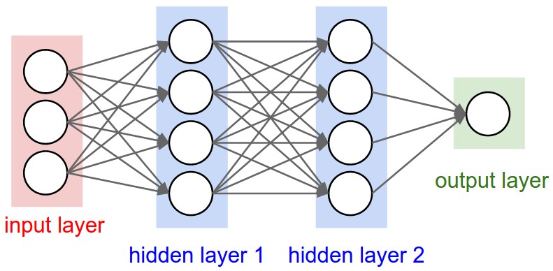
The representation power of the neural network depends on the number of hidden layers (depth). The name “deep” learning comes from this depth. Notice the connections in the figure. Every node in one layer is connected to every other node in the next or previous layer, but there are no connections between the nodes in the same layer. This kind of layers are called Fully connected layers. Also, notice the arrow pointing in the forward direction (looking from the input to output). This means that the flow of information happens from the input to the output, hence the name Feed Forward Neural Network. The network can be seen as a collection of non-linear functions that are parameterized by the weights (connections between neurons).
Representation Learning is another important property of Neural Networks that should be understood. In a deep network, the raw input is transformed into a useful form/feature/representation, through a series of non-linear transformations. This representation is useful, in the sense that it is convinient for the network to use the input in this form and learn the best input-output mapping. Moreover, the inputs, which are physical phenomena like sound, image, etc., are complex, noisy and highly redundant. While learning to map inputs to outputs, the network automatically learns the best representation from complex raw inputs that helps the network to get the job done. The job I mentioned could be classification, regression, etc,.
Introduction to Keras
Keras is a minimalist, highly modular neural networks library, written in Python and capable of running on top of either TensorFlow or Theano. It was developed with a focus on enabling fast experimentation. Being able to go from idea to result with the least possible delay is key to doing good research.
Install keras via pip.
sudo pip install keras -ULet us learn keras by creating an MLP (Multilayer perceptron) to classify digits from MNIST dataset.
import numpy as np
from keras.datasets import mnist
from keras.models import Sequential
from keras.layers.core import Dense, Dropout, Activation
from keras.optimizers import SGD, Adam, RMSprop
from keras.utils import np_utils
batch_size = 128
nb_classes = 10
nb_epoch = 20
# the data, shuffled and split between train and test sets
(X_train, y_train), (X_test, y_test) = mnist.load_data()
X_train = X_train.reshape(60000, 784)
X_test = X_test.reshape(10000, 784)
X_train = X_train.astype('float32')
X_test = X_test.astype('float32')
X_train /= 255
X_test /= 255
print(X_train.shape[0], 'train samples')
print(X_test.shape[0], 'test samples')
# convert class vectors to binary class matrices
Y_train = np_utils.to_categorical(y_train, nb_classes)
Y_test = np_utils.to_categorical(y_test, nb_classes)
model = Sequential()
model.add(Dense(512, input_shape=(784,)))
model.add(Dense(512))
model.add(Dense(10))
model.add(Activation('softmax'))
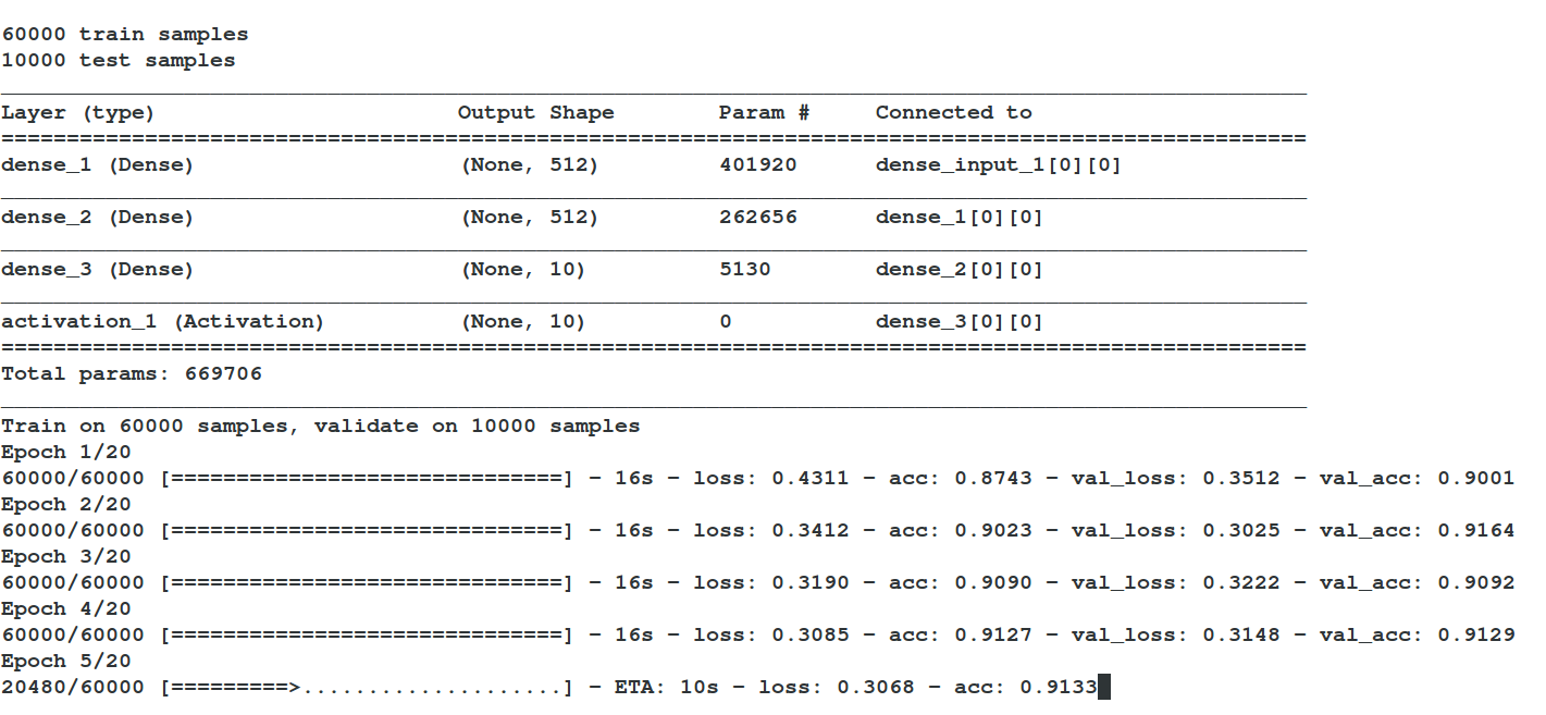
model.summary()
model.compile(loss='categorical_crossentropy',
optimizer=RMSprop(),
metrics=['accuracy'])
history = model.fit(X_train, Y_train,
batch_size=batch_size, nb_epoch=nb_epoch,
verbose=1, validation_data=(X_test, Y_test))
score = model.evaluate(X_test, Y_test, verbose=0)
print('Test score:', score[0])
print('Test accuracy:', score[1])