Unfolding RNNs

Update : Part 2 is now available at Unfolding RNNs II : Vanilla, GRU, LSTM RNNs from scratch in Tensorflow.

RNN is one of those toys that eluded me for a long time. I just couldn’t figure out how to make it work. Ever since I read Andrej Karpathy’s blog post on the Unreasonable Effectiveness of RNNs, I have been fascinated by what RNNs are capable of, and at the same time confused by how they actually worked. I couldn’t follow his code for text generation (Language Modeling). Then, I came across Denny Britz’s blog, from which I understood how exactly they worked and how to build them. This blog post is addressed to my past self that was confused about the internals of RNN. Through this post, I hope to help people interested in RNNs, develop a basic understanding of what they are, how they work, different variants of RNN and applications.

Warning : I have organized this post based on the structure of Chapter 10 of Ian Goodfellow’s book. Most concepts are directly taken from that chapter, which I have presented along with my comments. Do not be alarmed when you notice the similarities.

Recurrent Neural Networks are powerful models that are uniquely capable of dealing with sequential data, like natural language, speech, video, etc,. They bring the representation power of deep neural networks to the table, to understand sequential data and typically, make decisions. Traditional neural networks are stateless. They take a fixed size vector as input and produce a vector as output. RNNs, unlike any other networks before, have this unique property of being “stateful”. The internal state of the RNN captures information from an input sequence, as it reads the sequence, one step at a time.

Another interesting property of RNNs, is parameter sharing. Parameter sharing is a well known and widely used idea in Machine Learning. In convolutional neural networks, at each convol layer, a filter defined by same parameters, is applied throughout the image (convolution operation), to extract local features. Parameter sharing in RNNs, helps in applying the model to examples of different lengths. While reading a sequence, if we employ different parameters for each step during training, the model will never generalize to unseen sequences of different lengths.

Recurrence

Feed-forward neural networks and it’s variants like Convolutional Networks, can be easily understood because of their static architecture. A simple feed-forward neural network with a hidden layer, can be built by stacking one layer on top of another layer. The output at the last layer, \(\hat{y}\) is a non-linear funciton of the input, \(\hat{y} = f(x)\). f can be decomposed into layer-wise transformations as follows.

At each layer, we apply an affine transformation, followed by a non-linearity (sigmoid, hyperbolic tangent or ReLU). Finally, at the output layer, we apply softmax function, which provides normalized probabilities over output classes. We can express a neural network as a Directed Acyclic Graph(DAG), to understand the architecture and data flow.

Note : Unless otherwise mentioned explicitly, assume data flow from left to right, in the graphs below. Drawing arrows in Inkscape is a nightmare.

Pretty simple right? The input x, a vector of real numbers, is passed through multiple nodes of operations and transformed into class probabilities that we need for classification.

How are recurrent neural networks different from this network? Why can’t we draw an RNN as a DAG?

Because RNNs have cycles in them. To understand RNNs, we need to remove these cycles and draw the network as a DAG.

To that end, let us consider a dynamic system whose present state is a function of (depends on) the previous state. It can be expressed compactly, with cycles, as below:

This is a recursive/recurrent definition. The state at time ‘t’, \(s_{t}\) is a function (f) of previous state \(s_{t-1}\), parameterized by \(\theta\). This equation needs to be unfolded as follows:

External Signal, X

Consider a little more complex system, whose state not only depends on the previous state, but also on an external signal ‘x’.

The system takes a signal \(x_{t}\) as input during time step ‘t’, updates it’s state based on the influence of \(x_t\) and the previous state, \(s_{t-1}\). Now, let’s try to think of such a system as a neural network. The state of the system can be seen as the hidden units of a neural network. The signal ‘x’ at each time step, can be seen as a sequence of inputs given to the neural network, one input per time step. At this point, you should know that we are using the term “time step” interchangeably with steps in a sequence.

The state of such a neural network can be represented with hidden layer \(h_{t}\), as follows:

Unfolding

The neural network we just described, has recursion/recurrence in it. Let’s start calling it an RNN. It can be compactly represented as a cyclic circuit diagram, where the input signal is processed with a delay. This cyclic circuit can be unfolded into a graph as follows:

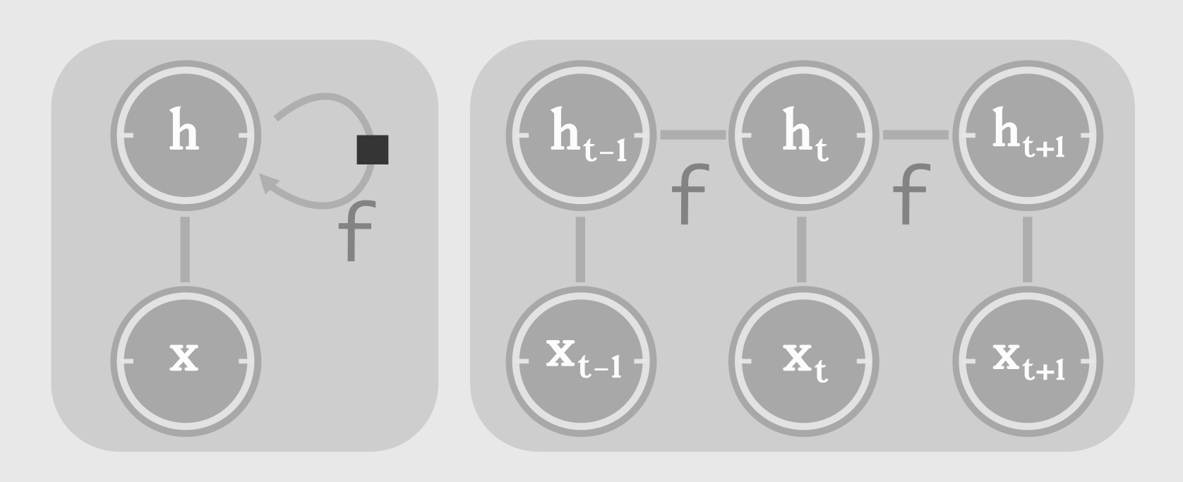Notice the repeated appliation of function ‘f’.

Let \(g_{t}\) be the function that represents the unfolded graph after ‘t’ time steps.

Now we can express the hidden state at time ‘t’, two ways:

• as a recurrence relation, as we have seen before

• as an unfolded graph

Forward Propagation

Now that we have a good picture of how RNNs function, let’s move on to more concrete aspects of it. Given a sequence of inputs \(\{x_1, x_2,... x_t\}\), how do you propagate it through an RNN? How do we handle the input, update the state and produce output at each step?

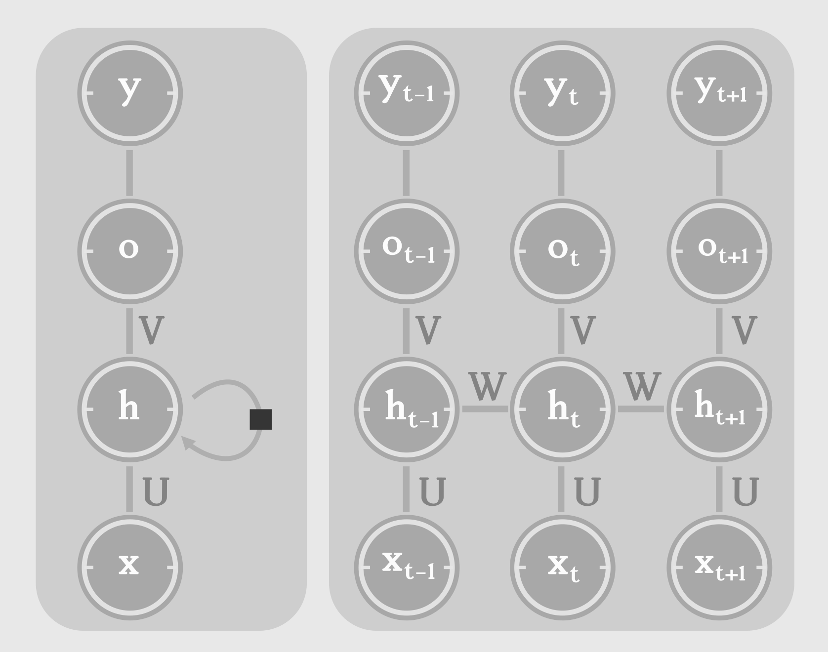
What do we know? The output at each step depends only on the state at each step, as the state captures everything necessary. The state is dependent on the current input and the previous state. The state at time ‘t’, \(h_t\) can be written as a function of previous state, \(h_{t-1}\) and current input \(x_t\) as follows:

The estimate, \(\hat{y_{t}}\) is typically a normalized probability over output classes. The loss compares the estimate with the ground truth (target).

Loss at time step ‘t’ is expressed as negative log likelihood of \(y_t\), given the input sequence till ‘t’, \(\{ x_1, ..., x_t \}\).

Being Markovian

A stochastic process has the Markov property if the conditional probability distribution of future states of the process (conditional on both past and present states) depends only upon the present state, not on the sequence of events that preceded it. A process with this property is called a Markov process.

The fixed-size hidden units used to represent the state of the network at each time step, is essentially a lossy summary of task-relevant aspects of the past sequence of inputs. RNNs are Markovian (ie.) the future states of the system, at any time ‘t’, depend entirely on the present state, not the past. In other words, the current state captures everything necessary from the past. During each time step, the internal state captures what is absolutely necessary to accomplish the task. What task? The task of maximising the conditional likelihood of output sequence given the input sequence, \(log P( \{ y_1, y_2,.. \} \mid \{ x_1, x_2,.. \} )\). We’ll revisit this in the next post, when I talk more about the objective function.

Vector to sequence

So far, we have seen a typical RNN, which takes an input at each step and produces an output at each step. There is a special category of RNN that takes a fixed-length vector as input and produces a series of outputs. An application of this architecture of RNN, is the task of image captioning. Given a fixed length vector which is typically the feature vector of the input image (we can use an MLP or a CNN to extract features of an image), our RNN need to generate a proper caption, word by word. The next word depends on the previous words and also the feature vector of the image (context vector).

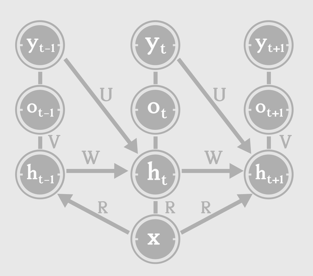
The context, ‘x’ influcences the network by acting as the new “bias” parameter - \(x^{T}R\).

Seq2Seq Architecture

There are applications where we might need to map a sequence to another sequence of different length. Recall from previous discussions that a traditional RNN emits one output for one input, at each step. Take Machine Translation for example. A sentence in English doesn’t necessarily translates to a French sentence of the same length. The Encoder-Decoder model or the Sequence to Sequence (seq2seq) model, consists of two RNNs : an encoder and a decoder. The encoder processes the input sequence. The encoder doesn’t emit an output at each step. Instead, it just takes the input sequence, one word at a time and tries to capture task-relevant information from the sequence, in it’s internal state. The final hidden state should ideally be a task-relevant summary of the input sequence. This final hidden state, is called the context or thought vector.

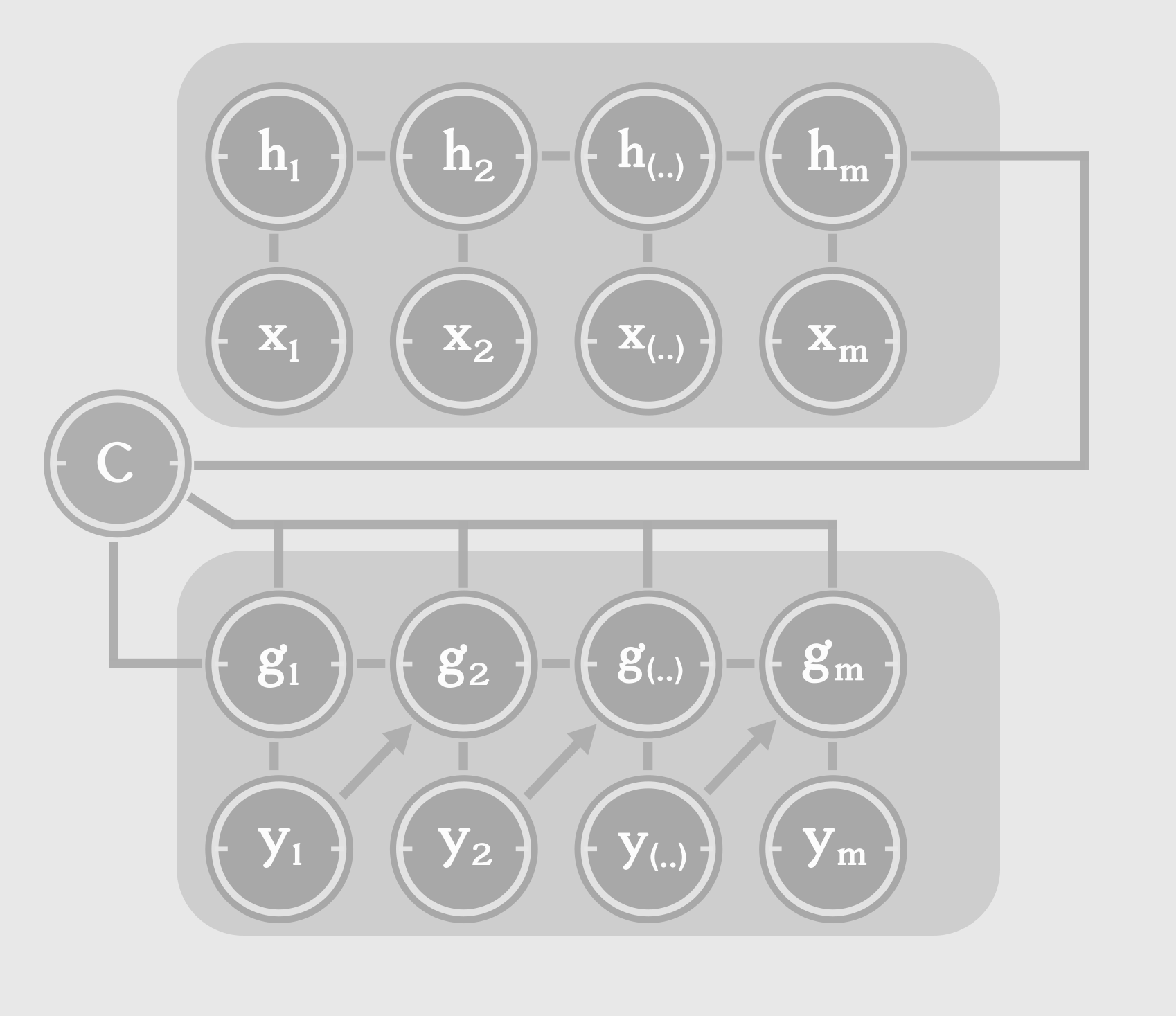
The context acts as the only input to the decoder. It can be connected to the decoder in multiple ways. The initial state of the decoder can be set as a function of the context or the context can be connected to the hidden states at every time step, or both. It is important to note that the hyperparameters of the encoder and decoder can be different, depending on the type of input and output sequences. For example, we can set the number of hidden units for encoder to be different than that of the decoder.

Bidirectional RNN

The RNNs we have seen so far, have a “causal” structures, (ie.) the present is influenced by the past, but not the future. The state of the system depends on the previous inputs, state, \(s_{t} = f(x_t, x_{t-1}, .. x_1)\). There is special category of RNN, in which the state of the system at time ‘t’ and therefore the output at ‘t’, \(o_t\), depends on not only on inputs from the past, but also on the inputs from the future. This is confusing right? Let’s forget about the past and future. Consider a input sequence, x = \({x_1, x_2, .., x_i,... x_n}\).

At step i, we have 2 hidden states - \(h_i\) and \(g_i\). \(h_i\) captures the flow of information from left to right \({x_1,x_2,...x_i}\), while \(g_i\) captures the information from right to left \({x_{i+1}, ... x_n}\). This kind of RNN, capable of capturing information from the whole sequence, is known as a Bi-directional RNN. As the name says, it has 2 RNNs in it, for processing the sequence from either directions. At each step i, we have information from the whole sequence. Where is this applicable?

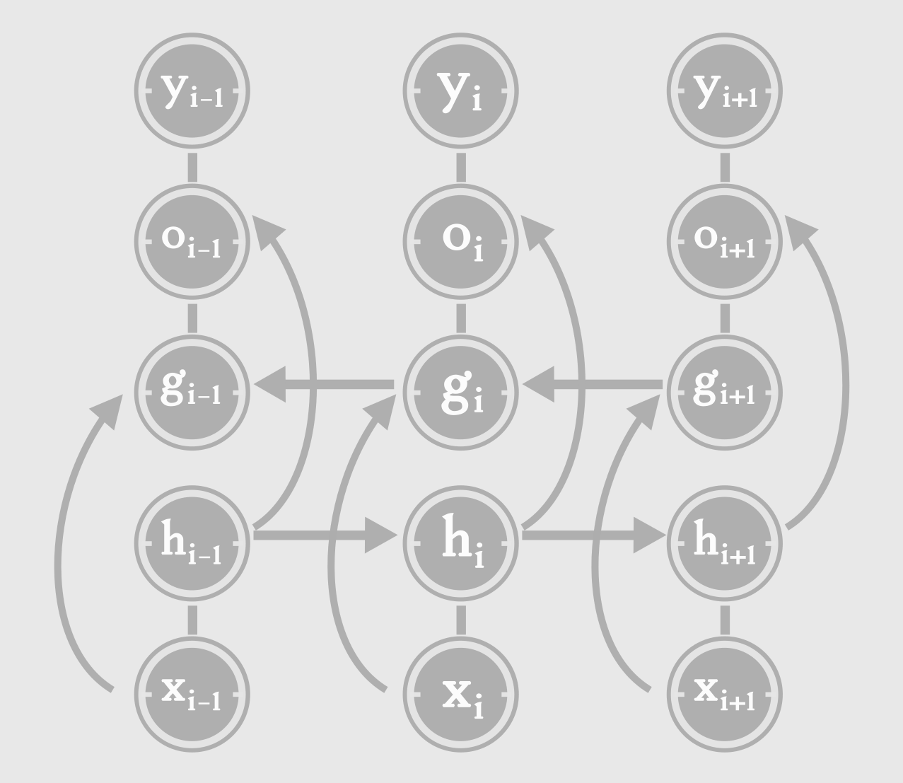
In speech recognition, we may need to pick a phoneme at step i, based on inputs from i+1, i+2,… We may even have to look futher ahead, and gather information from words in the future steps, in order for the phoneme at step i, to make linguistic sense.

Going Deeper

We need to be careful visualizing depth in an RNN. An RNN when unrolled can be seen as a deep feed-forward neural network. From this perspective, depth equals the number of time steps. Now consider a single time step ‘t’.

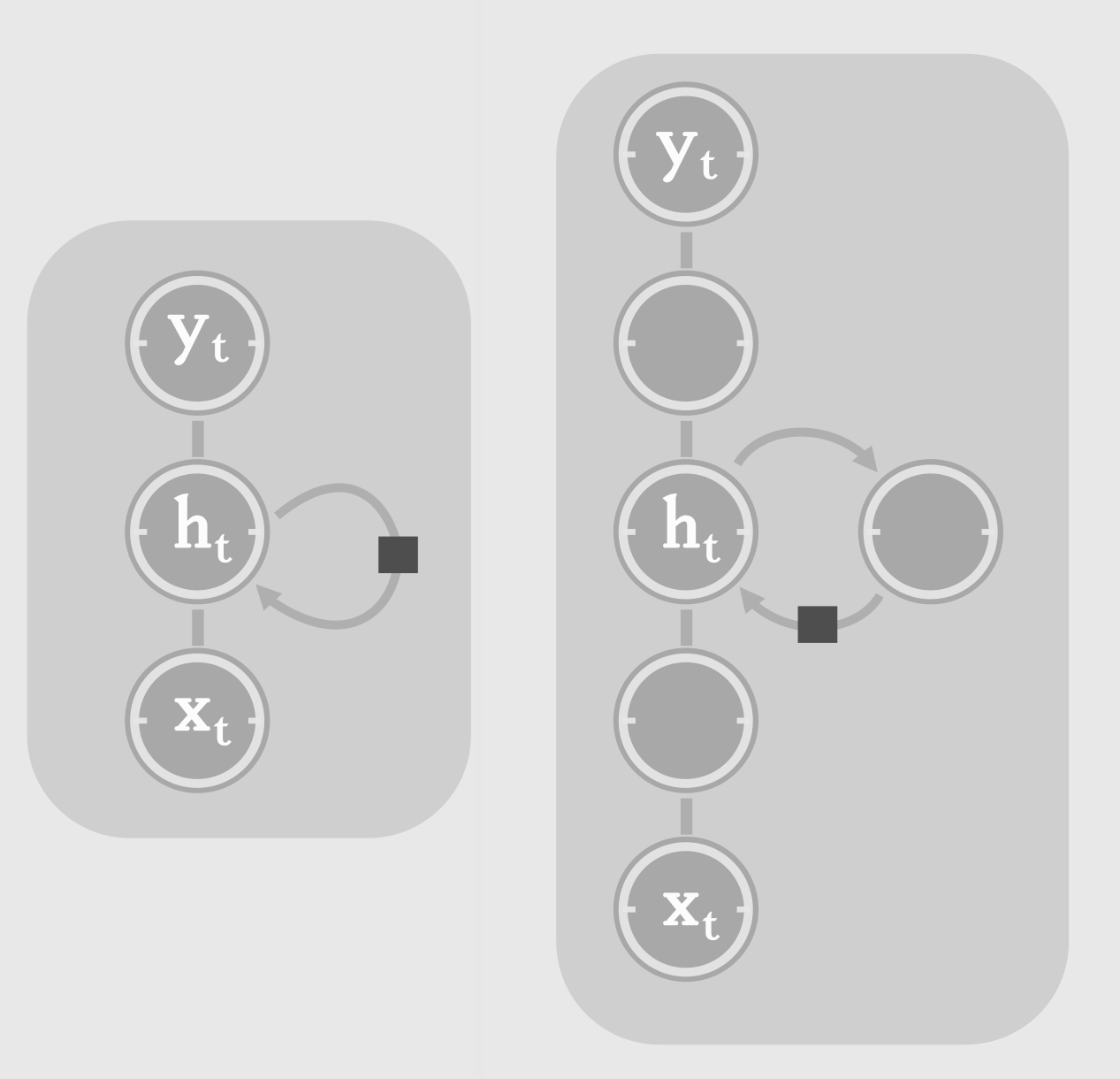
We can make computation at each time step, deeper by introducing more hidden layers. This type of RNN is known as Stacked RNN or more commonly, deep RNN. Typically, we have multiple layers of non-linear transformations, between hidden to hidden connections. This enables the RNN to capture higher level information (features composed of simpler features) from the input sequence, and store it as the state of the system. With great depth comes greater difficulty in training. Deeper RNNs take more time to train. But they are better in any of the tasks we have discussed, than shallow RNNs. And hence, in practice most people tend to use Stacked (multi-layer) RNNs.

Reference

1. Unreasonable Effectiveness of RNNs
2. Introduction to RNNs
3. Ian Goodfellow’s book
4. Deep Learning Book - chapter 10
5. Parameter Sharing in CNN

That’s it for now. I have covered the basics of RNN, selectively omitting a few important sections, like attention mechanism and teacher forcing, which we’ll visit in the future posts. In the next post, I will try to focus on the following:

• Sequence Loss
• Backpropagation through time
• Computing the gradient
• LSTM and GRU units
• Memory Networks

Don’t think twice about leaving a comment! Just do!

Update : Part 2 is now available at Unfolding RNNs II : Vanilla, GRU, LSTM RNNs from scratch in Tensorflow.