Pandas is a data manipulation and analysis library for python. It is heavily used by the Machine Learning community to clean, transform, and analyze structured data.

Why should you read this post?

I’ve been using pandas for working with structured data like Electronic Health Records (EHR), insurance claims, sensory data from wearables, etc. Pandas is a powerful data manipulation library that I’ve been consistently under-utilizing. In this post, I describe a list of pandas functions that I wish I knew about when I started with Data Science. If you are someone who works with data for a living you might find this useful.

Select features from file

Sometimes csv files contain too much information. Too many irrelevant columns. I used to read the whole file into memory and then get rid of the irrelevant columns. Instead, we could read only the useful columns from the file.

Consider the example of Melbourne housing prices data. Say we are interested in the following features:

Suburb
Rooms
Landsize
BuildingArea
YearBuilt
Price

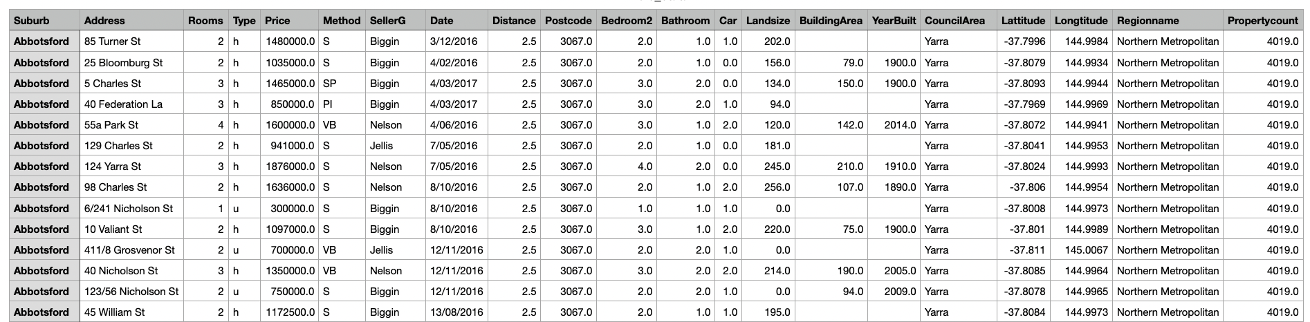
usecols option read_csv allows us to specify which columns we are interested in.

pd.read_csv("melb_data.csv",
            usecols=["Suburb", "Rooms", "Landsize", "BuildingArea", "YearBuilt", "Date", "Price"])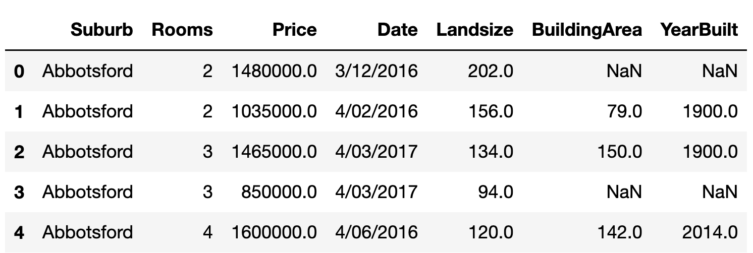

Parse Date as datetime data type

pandas by default parses columns containing date as the generic “object” type. We could take control of how it is parsed by using the parse_date option in read_csv.

df = pd.read_csv("melb_data.csv",
                   usecols=["Suburb", "Rooms", "Landsize", "BuildingArea", "YearBuilt", "Date", "Price"],
                    parse_dates=["Date"], dayfirst=True)
df.dtypes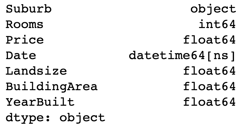

Dealing with Missing values

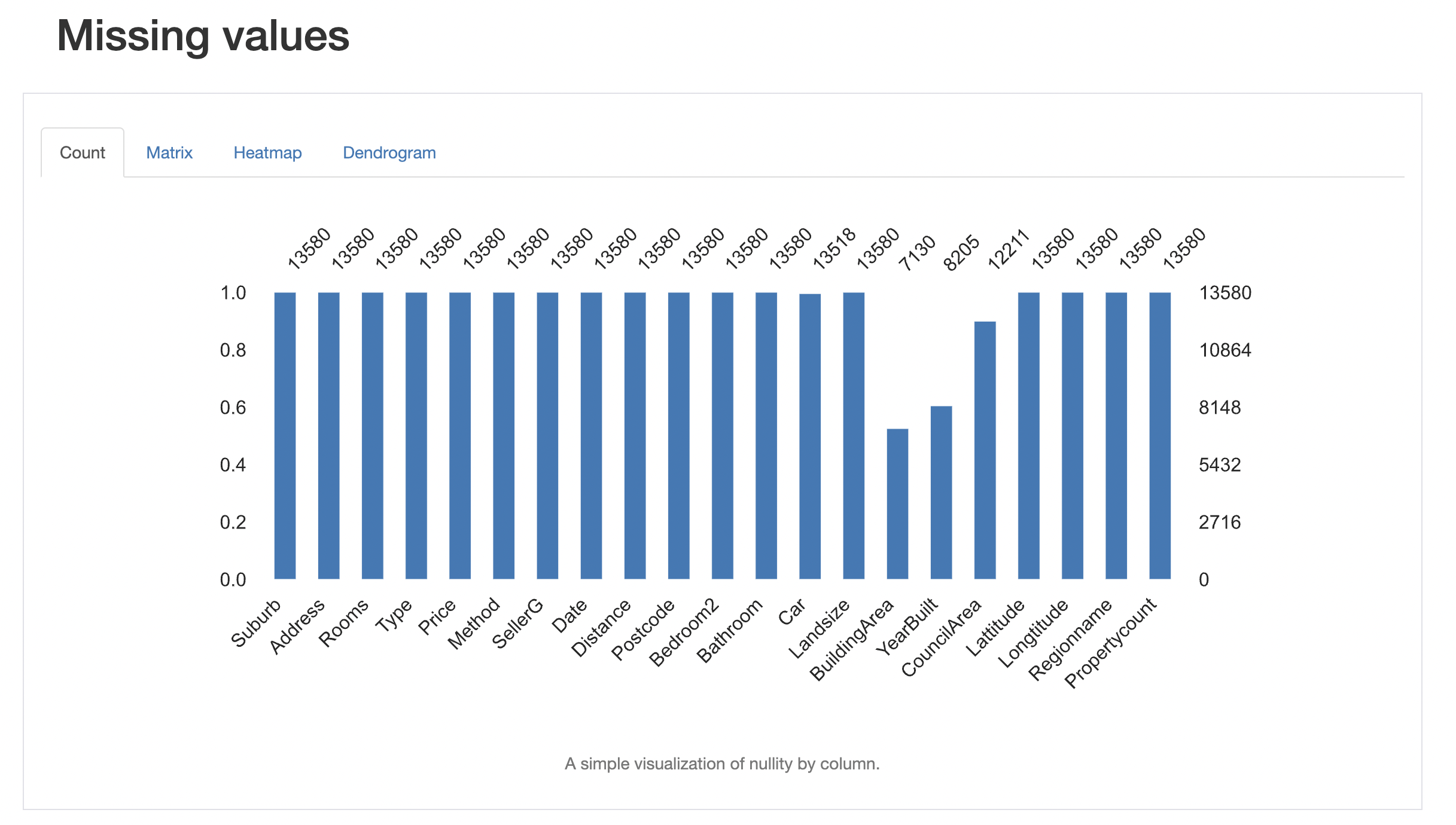
You may have noticed several NaN (missing) values in the data frame. We can decide to remove the rows with missing data or fill them in depending on the situation. There are many ways to fill in the missing values. We could fill in with average (mean, median) or most likely values (mode). Or we could use the values from the neighboring rows. Back-fill bfill fills in using the value from the next rows. Forward-fill ffill fills in using the value from the previous rows.

df.BuildingArea.fillna(method="ffill")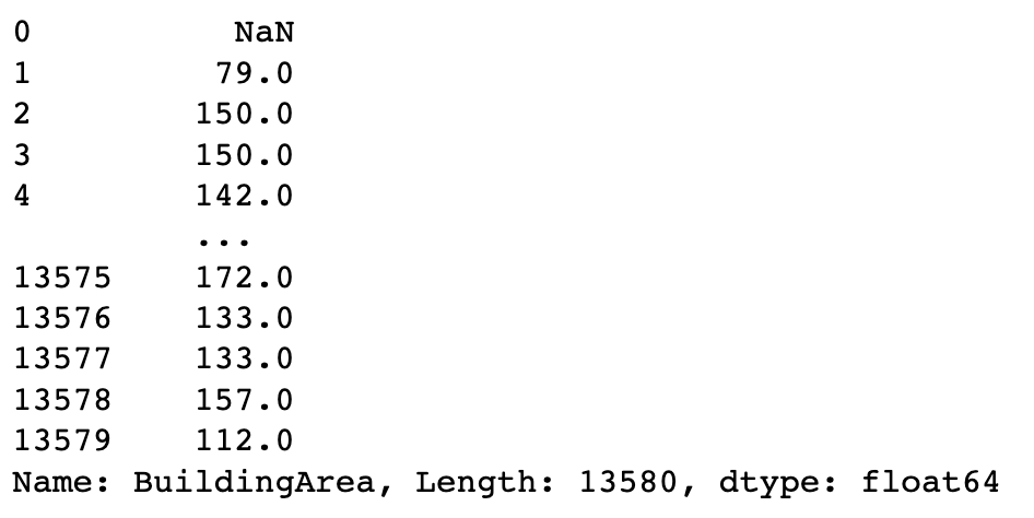

df.BuildingArea.fillna(method="bfill")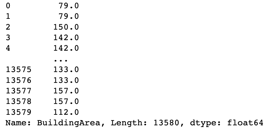

df.BuildingArea.fillna(df.BuildingArea.mean().item())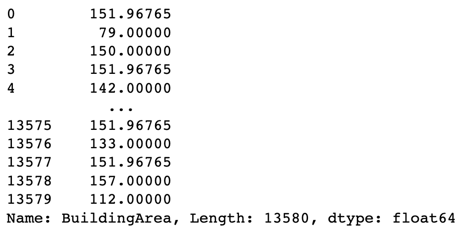

Filtering data

Almost every time I perform data analysis, I use conditions to filter out rows. Often I end up having to use multiple conditions leading to long, awkward lines of code.

df[(df.BuildingArea < 150) & (df.YearBuilt > 2000.) & (df.Rooms == 1)]

Alternatively, we could use df.query and enter our conditions as a string.

df.query("BuildingArea < 150. & YearBuilt > 2000. & Rooms == 1")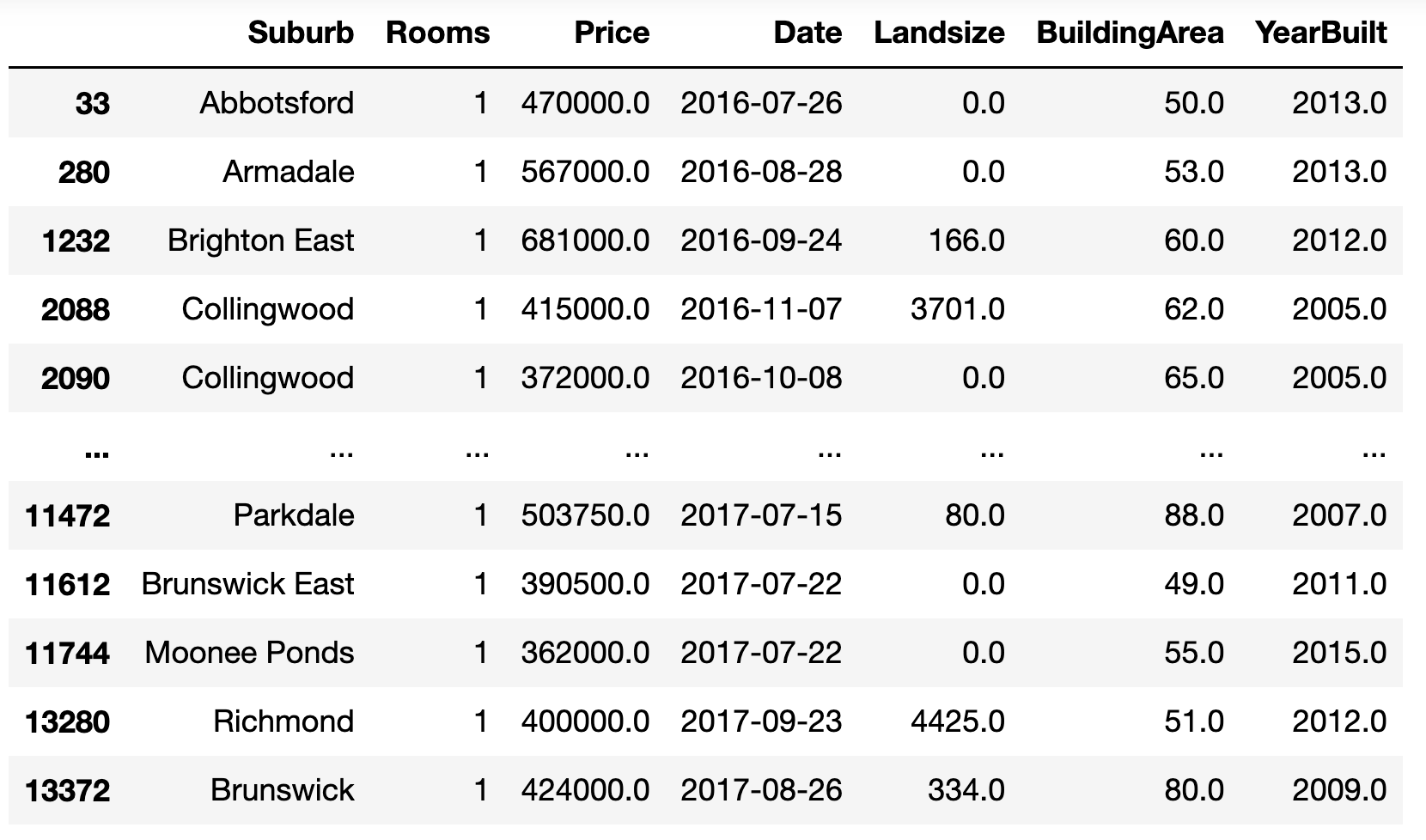

df.query("BuildingArea == Landsize").head()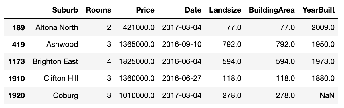

Is it in my list?

Here is another one that I use a lot. Let us say we are interested in a limited list of suburbs. How do we filter out the rest of the suburbs?

df[df.Suburb.isin(["Ashwood", "Altona North", "Coburg"])]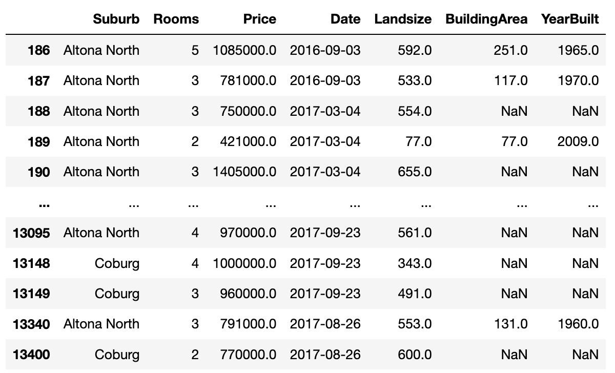

String Operations

pandas offers string-specific functionalities using a str accessor. There are methods equivalent to python’s string manipulation methods like lower, upper, strip, isalpha, find, index, split, and regex-based functions like match, search, and extractall (equivalent to re.findall). You can find a lit of string methods supported by pandas here.

df[df.Suburb.str.startswith("A")]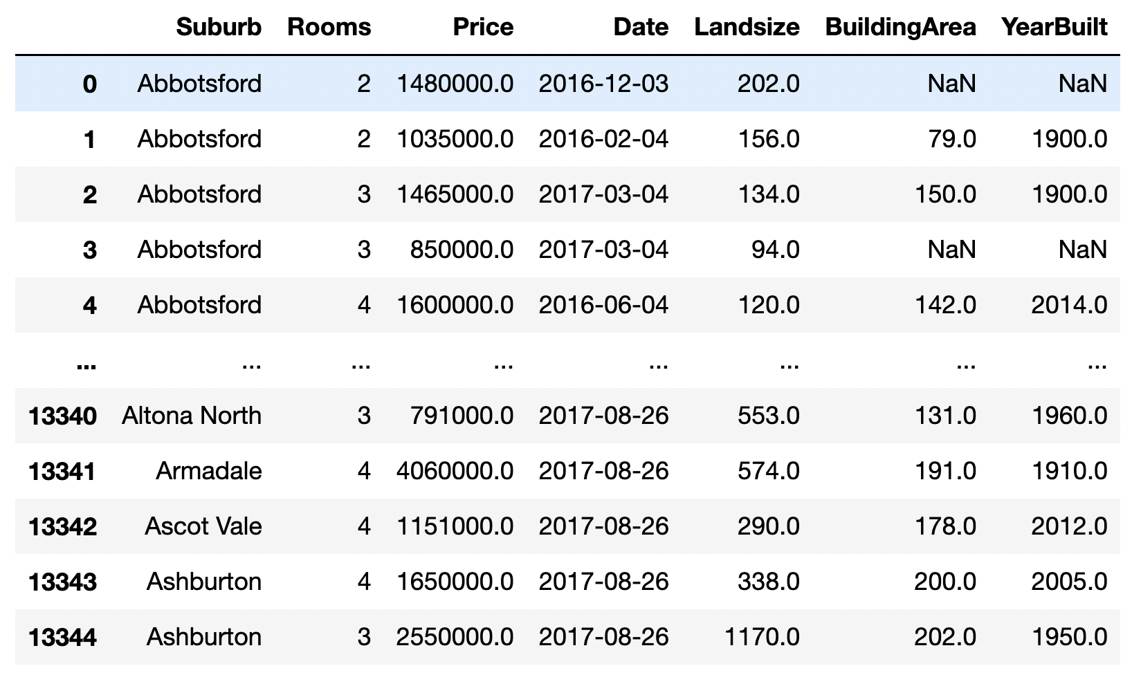

Date operations

pandas allows you to work with Date type objects using the dt accessor. pandas.Series.dt can be used to access date, hour, day, month, year, etc, from a Datetime object. It also supports many operations on Datetime objects like floor, ceil, normalize etc,.

df[df.Date.dt.year == 2016]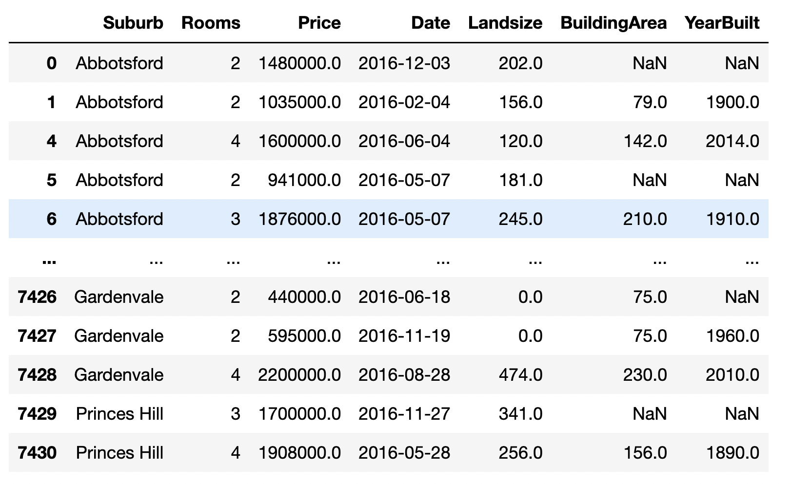

Group and Summarize

Groupby splits the data into different groups given a column. Using multiple columns to group will create a hierarchy of groups. The example below groups the data by “Regionname” and “Suburb” and summarizes the “Landsize” values within these groups.

df.groupby(["Regionname", "Suburb", ])[["Landsize"]].sum()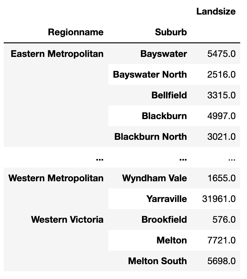

Ranking and Sorting

During data analysis, we’ll be interested in ranking entries in the data frame based on a variable of our choice. Looking at the extremes in the housing market might reveal interesting patterns. In the example below, we rank the housing entries based on their market price.

df["RankByPrice"] = df["Price"].rank(method="max")

Instead, we could just sort the entries based on one or more columns.

df_sane.sort_values(by=["BuildingArea", "Landsize"], ascending=False)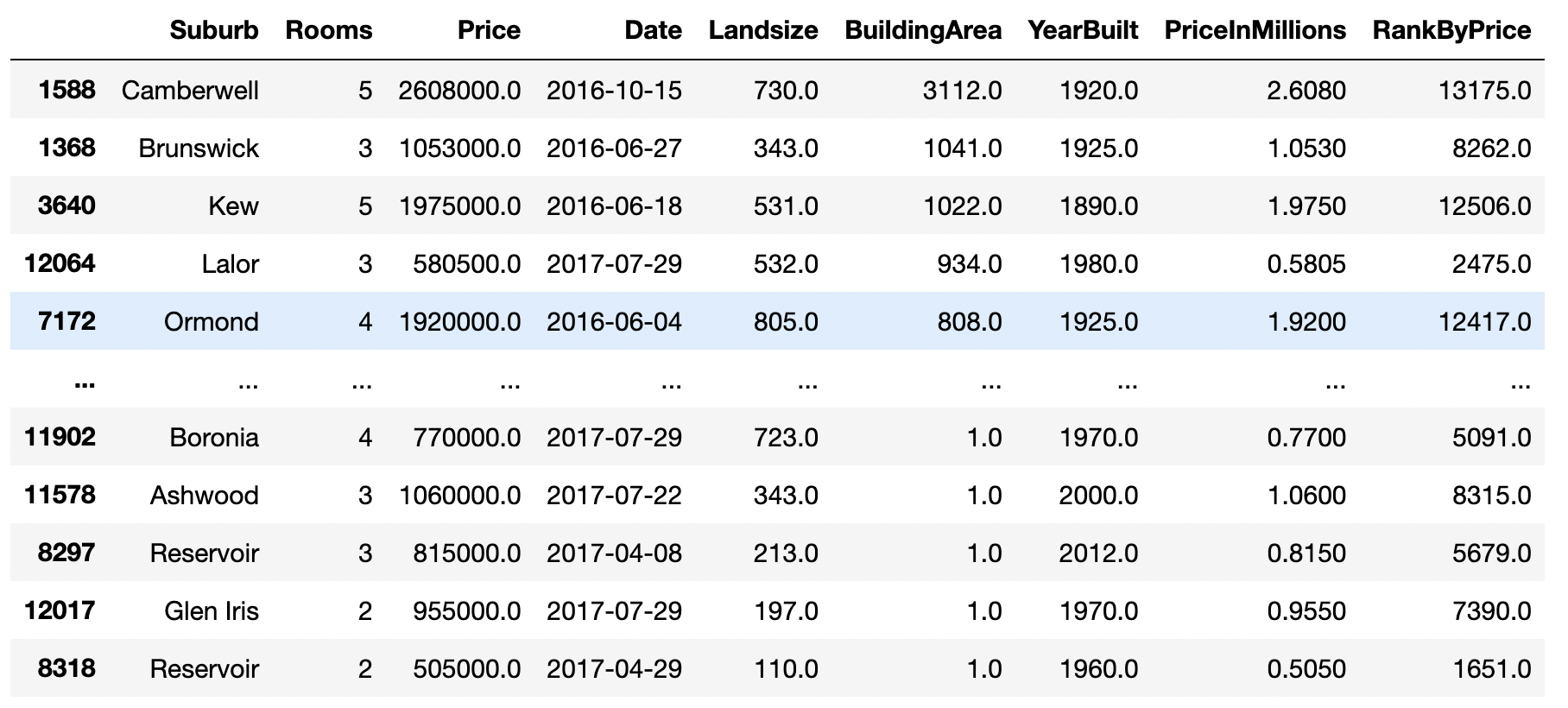

Correlation

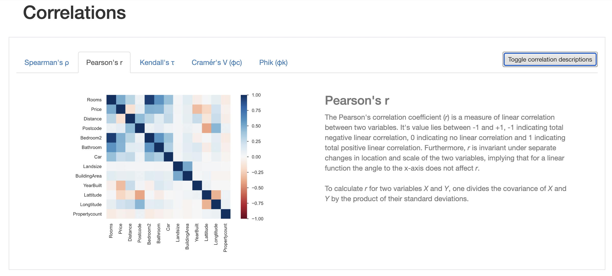
pandas has a handy function to calculate pair-wise correlation between variables. The correlation matrix is a good indicator of which features are useful (strong correlation with target variable) and which features are correlated with each other.

import seaborn as sns

corr = df.corr()
sns.heatmap(corr, cmap="Blues", annot=True);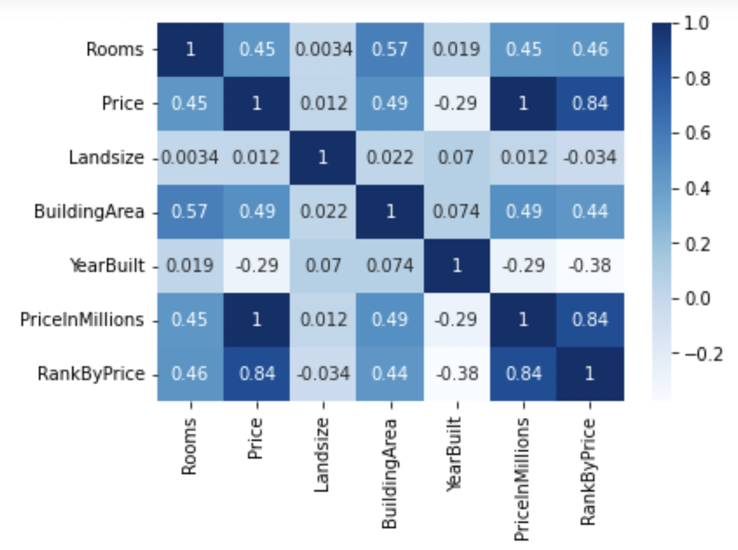

Combining data

When working with data from multiple sources, there is a need to combine them after cleaning and transformation. Pandas has functions to merge, join, append and concat data. merge and join are different ways of doing the same thing. merge performs a database-style join on data frames. concat and append perform concatenation of data frames along a particular axis.

In the code below,

land_size = df.groupby(["Regionname", "Suburb", ])[["Landsize"]].sum()
building_area = df.groupby(["Regionname", "Suburb",])[["BuildingArea"]].sum()
pd.merge(land_size, building_area, left_index=True, right_index=True)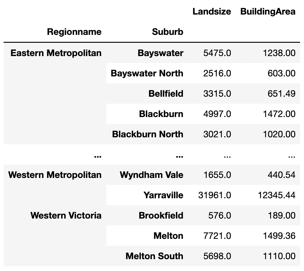

reset_index removes “Regionname” and “Suburb” as indices. Now to perform merge we need to explicitly include column names. The merge operation removes the indexes from the resulting data frame. Doing a merge on two unindexed data frames gives the same result.

pd.merge(land_size, building_area.reset_index(),
         left_index=True,
         right_on=["Regionname", "Suburb"])
pd.merge(land_size.reset_index(), building_area.reset_index(),
         on=["Regionname", "Suburb"])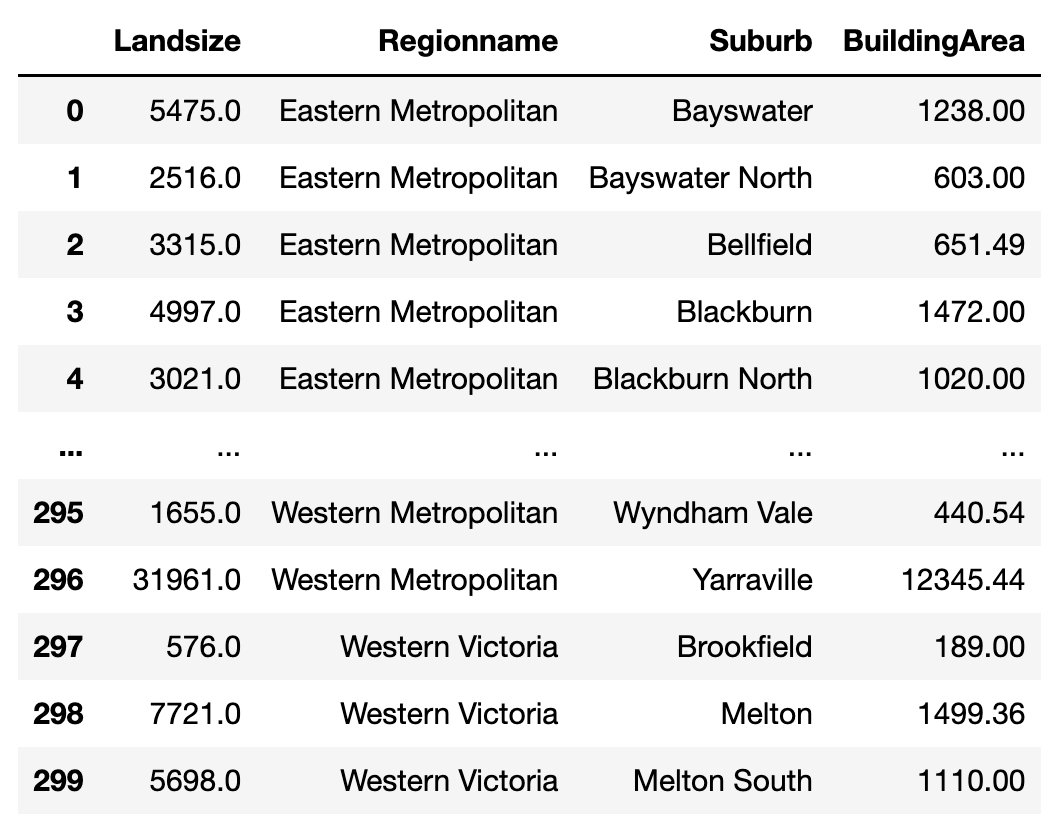

We can do sql-like merges using left, right, inner and outer methods.

pd.merge(land_size.reset_index(),
         building_area.reset_index().head(),
         how="left")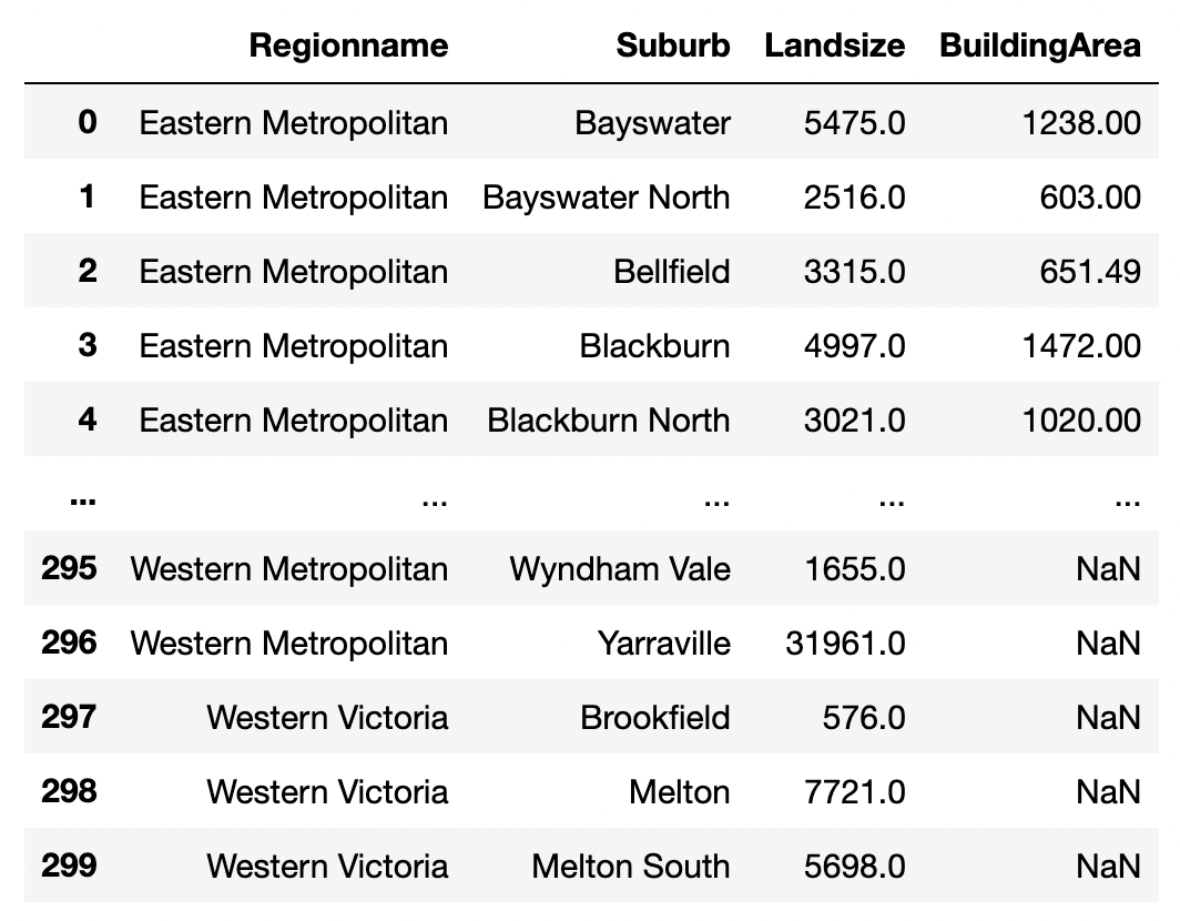

pd.merge(land_size.reset_index().head(),
         building_area.reset_index(),
         how="inner")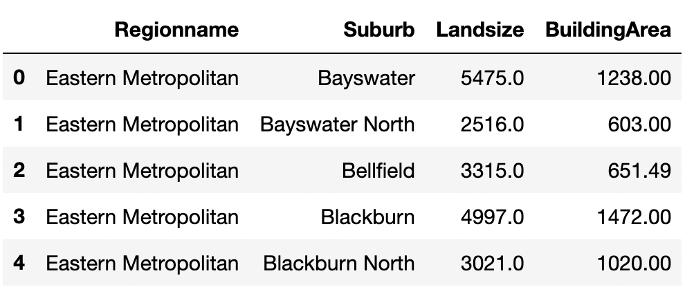

Setting indicator=True lets us know how each row was merged.

pd.merge(land_size.reset_index().head(),
         building_area.reset_index().tail(),
         how="outer", indicator=True)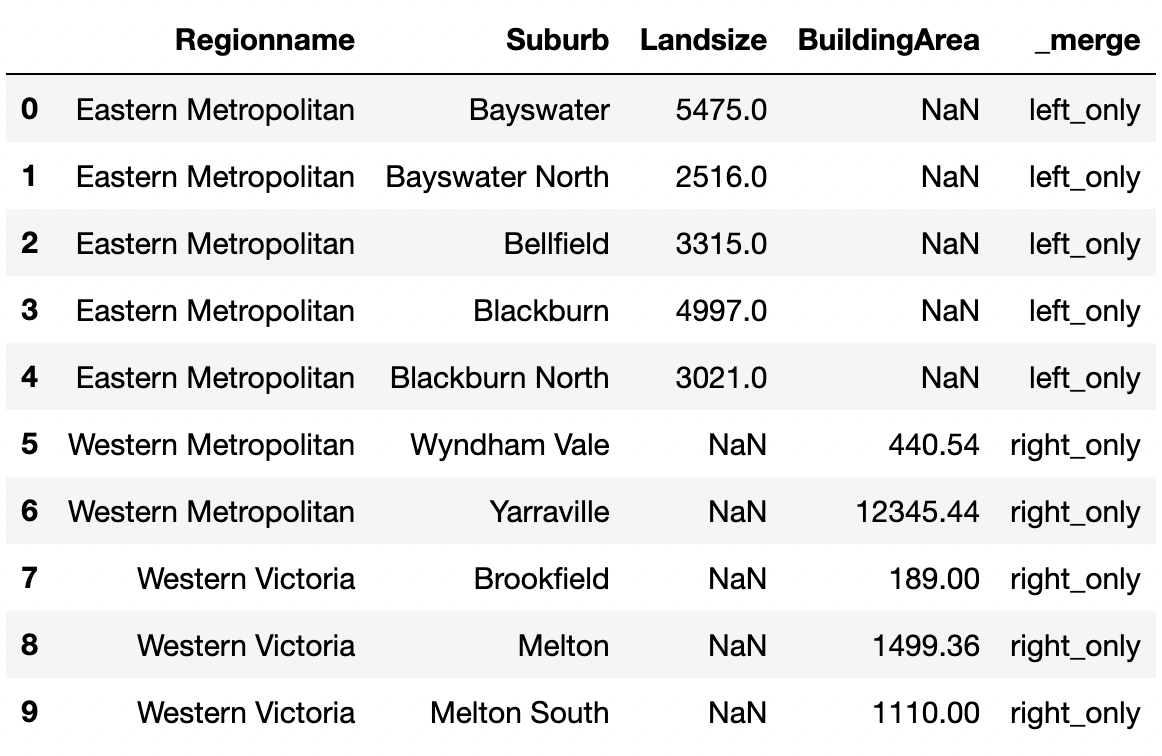

Concatenation is a simpler operation that combines two or more data frames row-wise or column-wise.

pd.concat([land_size, building_area])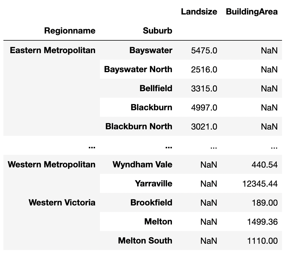

Concatenation work along the column axis using axis=1.

pd.concat([land_size, building_area], axis=1)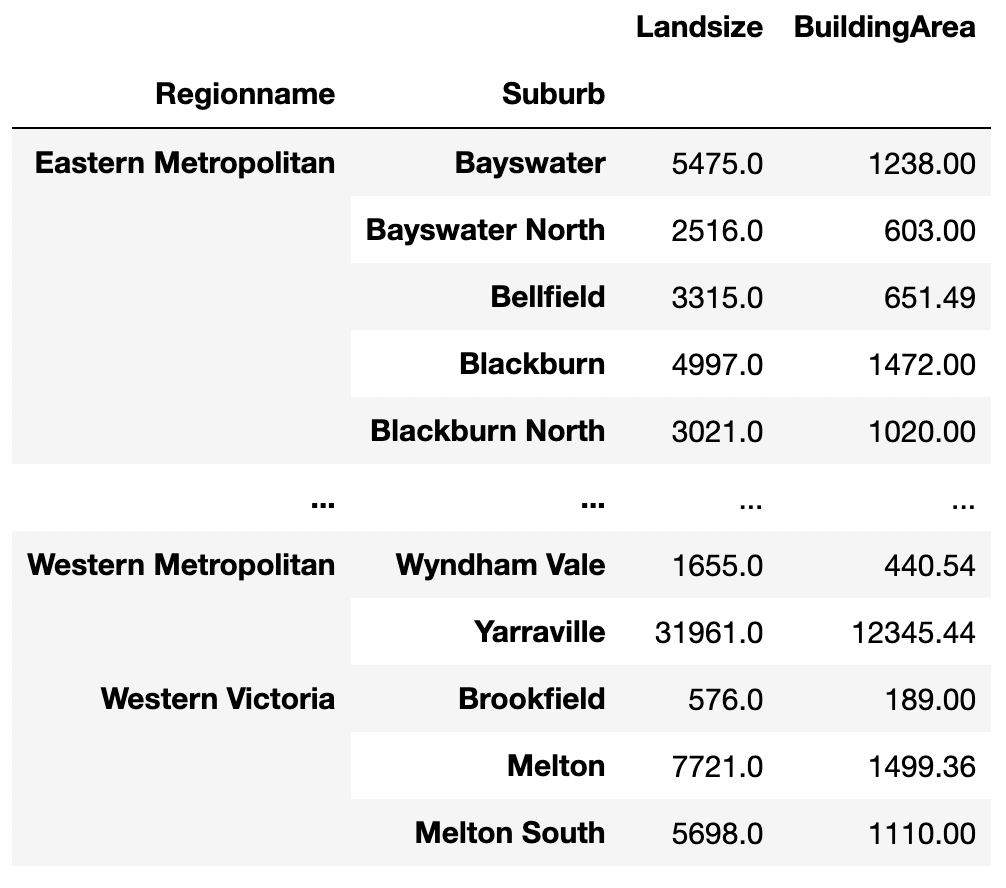

Contigency Tables

pd.crosstab takes an index and a list of columns as inputs and creates a simple cross tabulation between two or more factors. It creates a frequency table of factors. The frequency can be replaced by a different kind of summary by specifying a summarization function.

pd.crosstab(df.Suburb, [df.Rooms])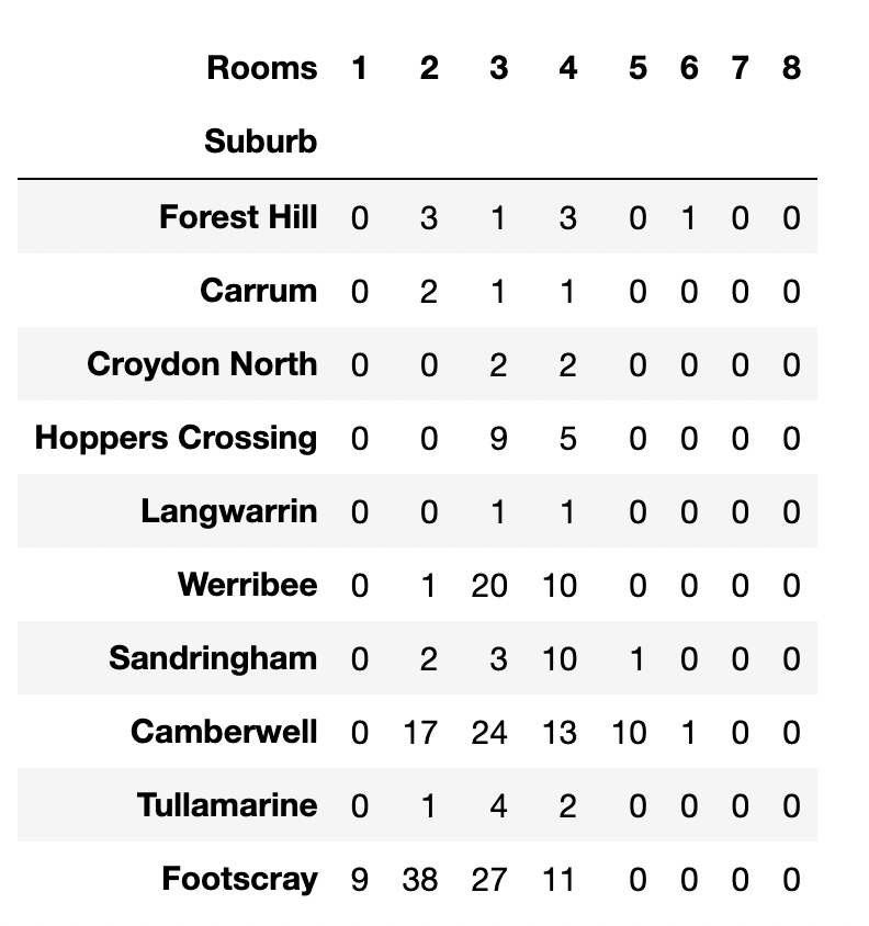

Multi-level data frames

It might be useful to group our entries based on, say the source of the data if we are acquiring and integrating data from different sources. Grouping like that creates a multi-level data frame.

pd.concat([land_size.reset_index(), building_area.reset_index()],
        keys=["land", "building"])

Profiling

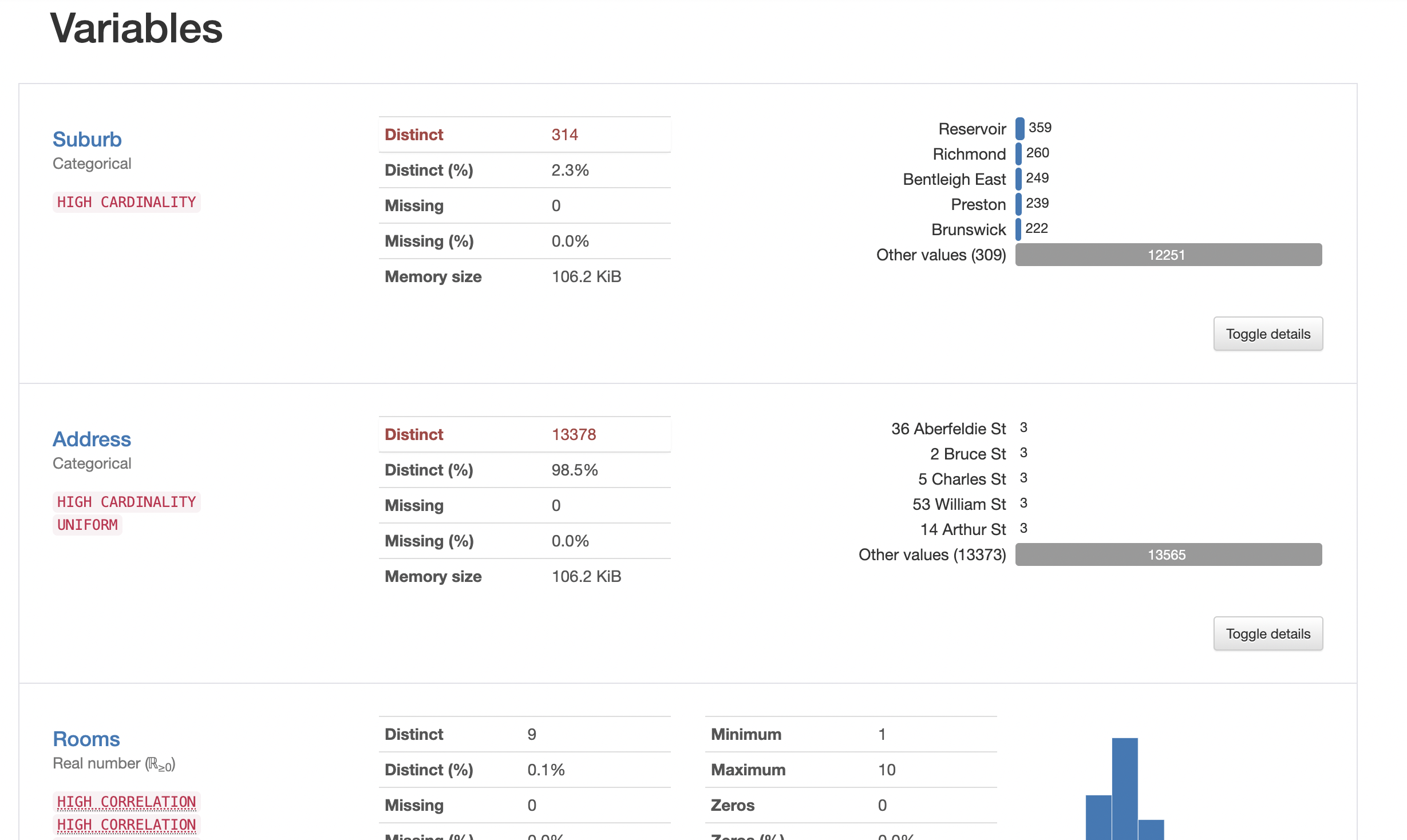
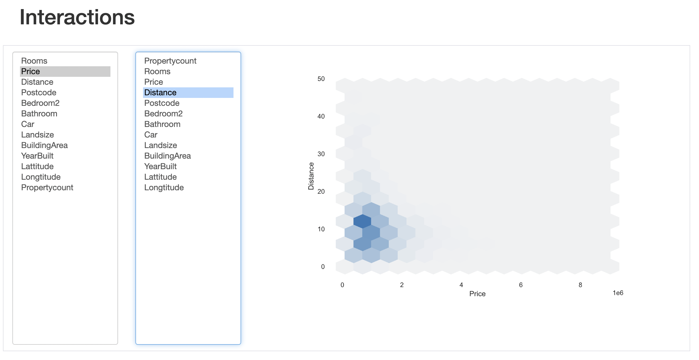
pandas_profiling is an external package that generates a detailed report on a pandas data frame. It generates a html report which includes tons of useful information such as global data statistics, variable statistics, missing value count, interaction between variables, correlation between variables, etc.

from pandas_profiling import ProfileReport

prof = ProfileReport(df)
prof.to_file(output_file='output.html')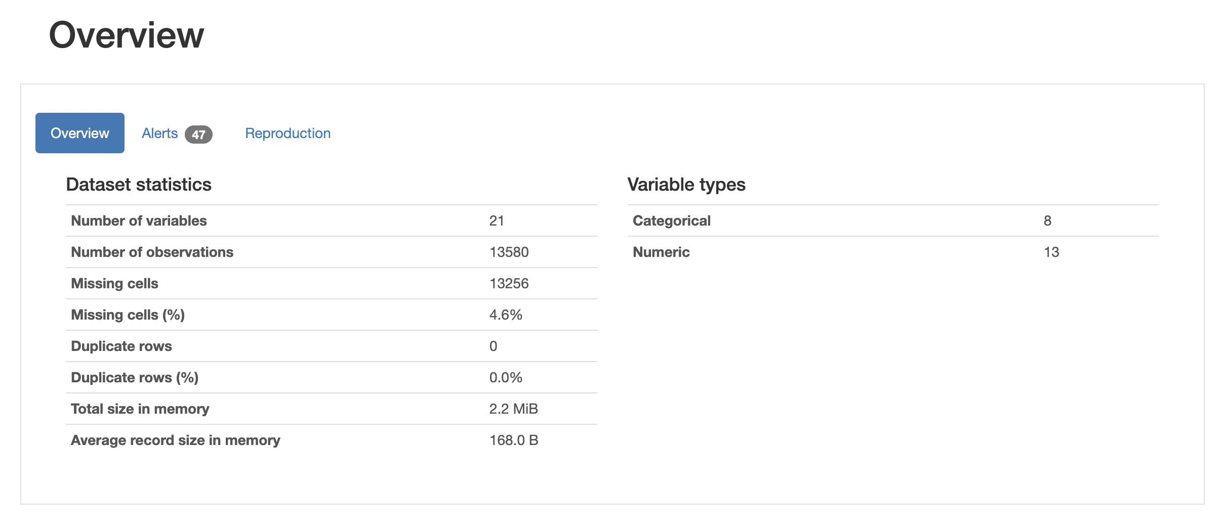

pandas is an incredibly powerful, flexible, and intuitive tool for working with structured data. I’m thinking of writing a follow-up blog that covers SQL-like functions in pandas and compares SQL queries with pandas functions.

That’s it for now. I hope one of these tricks helps you improve your workflow. See you soon with more.

If you got something to say leave a comment below.

Advanced Tricks in Pandas

Pandas functions that I wish I knew when I started