The first article in this series focused on the general mechanism of RNN, architectures, variants and applications. The objective was to abstract away the details and illustrate the high-level concepts in RNN. Naturally, the next step is to dive into the details. In this article, we will follow a bottom-up approach, starting with the basic recurrent operation, building up to a complete neural network which performs language modeling.
As we have seen in the previous article, the RNNs consist of states, which are updated every time step. The state, at time step t, is essentially a summary of the information in the input sequence till t. At each t, information flows from the current input and the previous state, to the current state. This flow of information can be controlled. This is called the gating mechanism. Conceptually, a gate is a structure that selectively allows the flow of information from one point to another. In this context, we can employ multiple gates, to control information flow from the input to the current state, previous state to current state and from current state to output. Based on how gates are employed to control the information flow, we have multiple variants of RNNs.
In this article, we will understand and implement the 3 most famous flavors of RNN - Vanilla, GRU and LSTM. The vanilla RNN is the most basic form of RNN. It has no gates, which means, information flow isn’t controlled. Information that is critical to the task at hand, could be overwritten by redudant or irrelevant information. Hence, vanilla RNNs aren’t used in practice. Though, they are very useful in learning RNNs. GRU and LSTMs consist of multiple gates that enable selective forgetting or remembering information from sequence. Let’s start with vanilla RNN.
Vanilla RNN
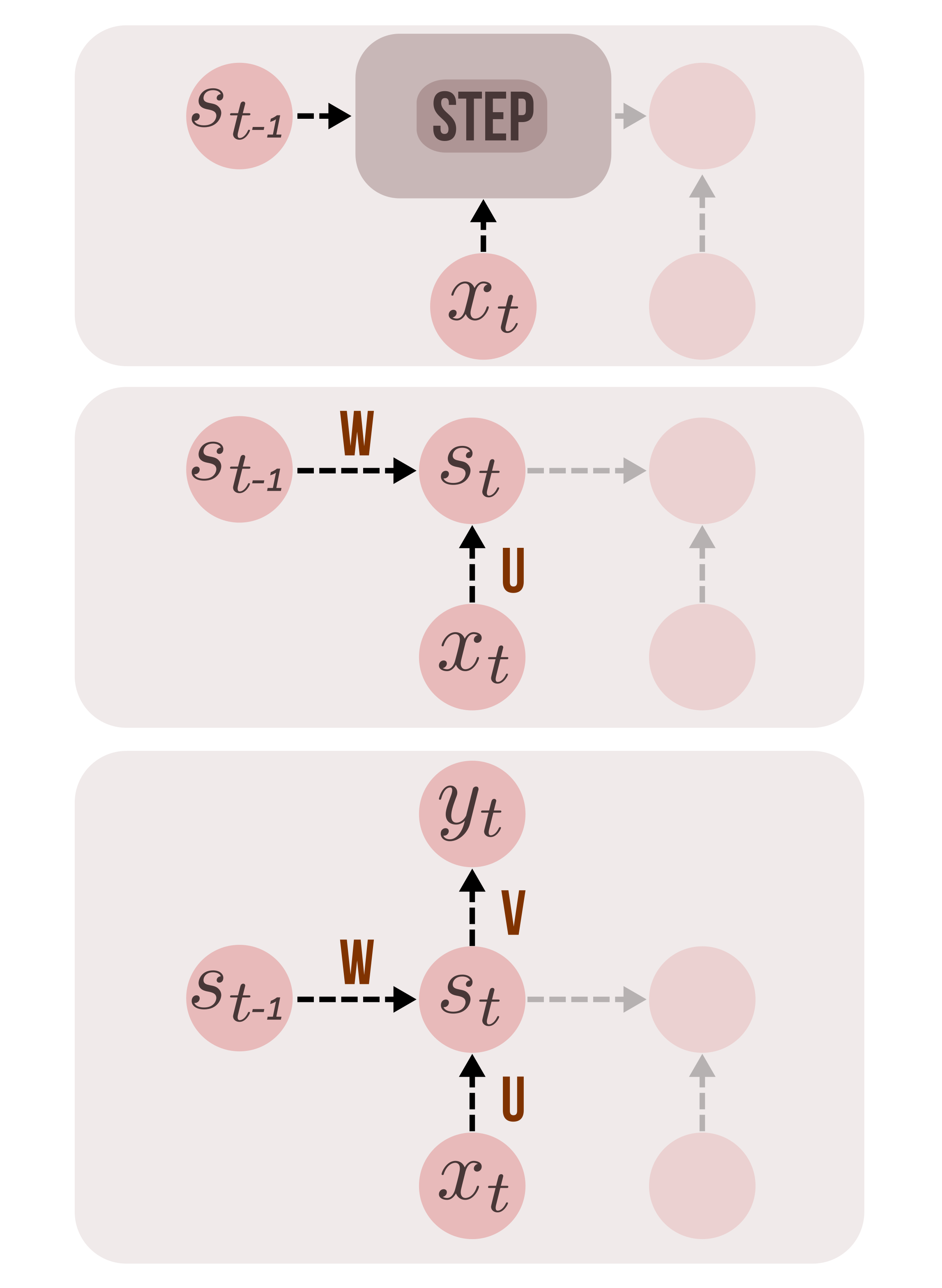
At each time step, the current state is the sum of linear transformations of current input and the previous state, parameterized by weight matrices U and W respectively, followed by a non-linearity (hyperbolic tangent). The output at t, is a similar linear transformation of current state \(s_t\), followed by a softmax, which converts logits into normalized class probabilities. The class prediction at each time step, \(\hat{y_t}\), assuming that we are dealing with a classification problem (sequence labeling), is calculated with the argmax function applied on \(o_t\).
At time step t,
\[s_t = tanh(Ux_t + Ws_{t-1})\\ o_t = softmax(Vs_t)\\ \hat{y_t} = argmax(o_t)\\\]Recurrence in Tensorflow
We now know what happens during each time step in a vanilla RNN. How do we implement this in tensorflow? The length of the input sequence varies for each example. A computational graph defined in tensorflow should run the recurrence operation over each item in the input sequence, one step at a time. It should be able to handle variable length sequences. In other words, it should dynamically unfold the recurrent operation T times for each T lengths of input sequences. This requires a loop in the computational graph. Tensorflow provides scan operation, precisely for this purpose. Let us take a look at tf.scan.
tf.scan(fn, elems, initializer) # scan operation
def fn(st_1, xt): # recurrent function
    st = f(st_1, xt)
    return st
The usage is fairly simple. fn is the recurrent function that runs T times. elems is the list of elements of length T- the input sequence, over which fn is applied. During each iteration, the state of the system is calculated as a function of current input, xt and the previous state, st_1. This state, st is passed to the next recurrent operation at t+1. initializer is a parameter that sets the initial state of the system. The states and the inputs discussed here, are basically just vectors of fixed length.
Language Modeling
Before jumping into the code, let me introduce the task of language modeling (RNNLM). The objective of language modeling is to capture the statistical relationship among words in a corpus, by learning to predict the next word, given a word. Based on which we will generate text one word at a time. I’ve used the term “word” here, but we will work with characters, simply because it is easier to work with data that way. The vocabulary will be fixed and small, and we don’t have to deal with rare words. Consider the small piece of text below, extracted from Paul Graham’s blog.
November 2016If you’re a California voter, there is an important proposition on your ballot this year
During preprocessing, we convert the raw text into a structured form (See table below). The objective of the network is to observe the input x, one character at a time and produce the output sentence y, one character at a time.
| X (string) | Y (string) |
|---|---|
| November 2016If you’ | ovember 2016If you’r |
| re a California vote | e a California voter |
| r, there is an impor | , there is an import |
| tant proposition on | ant proposition on y |
| your ballot this yea | our ballot this year |
Based on the text corpus, we build a vocabulary of all the characters. We randomly assign an index to each of the character.
| id | ch | id | ch | id | ch | id | ch |
|---|---|---|---|---|---|---|---|
| 0 | ” | 25 | m | 50 | & | 75 | J |
| 1 | ≈ | 26 | - | 51 | o | 76 | / |
| 2 | l | 27 | < | 52 | t | 77 | — |
| 3 | ? | 28 | G | 53 | ) | 78 | Q |
| 4 | r | 29 | ’ | 54 | 4 | 79 | ( |
| 5 | é | 30 | } | 55 | T | 80 | , |
| 6 | w | 31 | k | 56 | X | 81 | c |
| 7 | 6 | 32 | \n | 57 | I | 82 | x |
| 8 | 2 | 33 | 58 | a | 83 | f | |
| 9 | z | 34 | { | 59 | s | 84 | j |
| 10 | ` | 35 | ^ | 60 | V | 85 | M |
| 11 | U | 36 | F | 61 | E | 86 | R |
| 12 | u | 37 | * | 62 | 3 | 87 | : |
| 13 | + | 38 | 0 | 63 | h | 88 | % |
| 14 | b | 39 | ] | 64 | [ | 89 | O |
| 15 | p | 40 | 8 | 65 | L | 90 | Z |
| 16 | 1 | 41 | d | 66 | . | 91 | 7 |
| 17 | P | 42 | D | 67 | # | 92 | _ |
| 18 | ! | 43 | @ | 68 | S | 93 | g |
| 19 | W | 44 | B | 69 | | | 94 | q |
| 20 | 9 | 45 | K | 70 | ² | 95 | ; |
| 21 | N | 46 | 5 | 71 | A | 96 | H |
| 22 | y | 47 | $ | 72 | > | 97 | n |
| 23 | C | 48 | Y | 73 | v | 98 | = |
| 24 | i | 49 | xa0 | 74 | e |
Using the vocabulary we built, we will now map the data (X,Y) from raw string format, to corresponding indices.
| X (indices) | Y (indices) |
|---|---|
| [ 21, 51, 73, 74, 25, 14, 74, 4, 33, 8, 38, 16, 7, 57, 83, 33, 22, 51, 12, 29 ] | [ 51, 73, 74, 25, 14, 74, 4, 33, 8, 38, 16, 7, 57, 83, 33, 22, 51, 12, 29, 4 ] |
| [ 4, 74, 33, 58, 33, 23, 58, 2, 24, 83, 51, 4, 97, 24, 58, 33, 73, 51, 52, 74 ] | [ 74, 33, 58, 33, 23, 58, 2, 24, 83, 51, 4, 97, 24, 58, 33, 73, 51, 52, 74, 4 ] |
| [ 4 80 33 52 63 74 4 74 33 24 59 33 58 97 33 24 25 15 51 4] | [80 33 52 63 74 4 74 33 24 59 33 58 97 33 24 25 15 51 4 52] |
| [52 58 97 52 33 15 4 51 15 51 59 24 52 24 51 97 32 51 97 33] | [58 97 52 33 15 4 51 15 51 59 24 52 24 51 97 32 51 97 33 22] |
| [22 51 12 4 33 14 58 2 2 51 52 33 52 63 24 59 33 22 74 58] | [51 12 4 33 14 58 2 2 51 52 33 52 63 24 59 33 22 74 58 4] |
We understand that the network reads inputs in the form of an array of indices. But the indices by themselves, carry no semantic meaning and hence, the network will have a hard time mapping input sentences to output sentences. This is where embedding comes in; more commonly known as word vector or word embedding. In this case, we will map the characters to low dimensional vectors of size state_size. This is done by creating an embedding matrix of shape [ vocab_size, state_size ] and selecting a row of the matrix by index of character. This matrix is initialized randomly and hence the embeddings are useless before training. But, as the training progresses, loss is gradually minimized, maximizing the objective (predicting next character correctly), the network learns useful task-relevant embeddings. If you find the topic of Word Embedding fascinating, you will love Sebastian Ruder’s blog. In the article On Word Embeddings, he provides a comprehensive guide to understanding Word Embeddings.
data.py reads raw text extracted from Paul Graham’s blog. If you are interested in how I extracted text from his blog, check out scraper.py. The steps mentioned above are followed in creating the dataset. Let us move on to building the model as a graph in tensorflow.
Placeholders
import tensorflow as tf
import numpy as np
xs_ = tf.placeholder(shape=[None, None], dtype=tf.int32)
ys_ = tf.placeholder(shape=[None], dtype=tf.int32)
init_state = tf.placeholder(shape=[None, state_size],
    dtype=tf.float32, name='initial_state')
Placeholders are entry points through which data can be fed to the graph, during execution. The inputs xs_ and outputs ys_ are arrays of indices, of symbols in vocabulary as discussed in the last section. The initial state of the network is created as a placeholder, init_state, which should be set during execution of graph. The shape of initial state is of form [ batch_size, state_size ].
Embedding
embs = tf.get_variable('emb', [num_classes, state_size])
rnn_inputs = tf.nn.embedding_lookup(embs, xs_)
The inputs are transformed into embeddings, using the embedding matrix, embs. embedding_lookup is a wrapper that basically selects a row of embs for each index in xs_, which is an array of indices.
tf.scan
states = tf.scan(step,
        tf.transpose(rnn_inputs, [1,0,2]),
        initializer=init_state)
The scan function builds a loop that dynamically unfolds, to recursively apply the function step, over rnn_inputs. The dimensions of tensor rnn_inputs, are shuffled, to expose the sequence length dimension as the 0th dimension, to enable iteration over the elements of the sequence. The tensor of form [batch_size, seqlen, state_size], is transposed to [seqlen, batch_size, state_size]. states returned by scan is an array of states from all the time steps, using which we will predict the output probabilities at each step.
Recurrence
xav_init = tf.contrib.layers.xavier_initializer
W = tf.get_variable('W', shape=[state_size, state_size],
     initializer=xav_init())
U = tf.get_variable('U', shape=[state_size, state_size],
     initializer=xav_init())
b = tf.get_variable('b', shape=[state_size],
     initializer=tf.constant_initializer(0.))
We define the weight matrices W, U and bias b, which parameterize the affine transformation given by \(Ux_t + Ws_{t-1} + b\). Note that bias is optional.
def step(hprev, x):
    return tf.tanh(
        tf.matmul(hprev, W) +
        tf.matmul(x,U) + b)
At time step t, the state given by \(s_t = tanh(Ux_t + Ws_{t-1})\), is calculated and passed to the next step.
Output
V = tf.get_variable('V', shape=[state_size, num_classes],
                    initializer=xav_init())
bo = tf.get_variable('bo', shape=[num_classes],
                        initializer=tf.constant_initializer(0.))
states_reshaped = tf.reshape(states, [-1, state_size])
logits = tf.matmul(states_reshaped, V) + bo
predictions = tf.nn.softmax(logits)
The parameters of output transformation, V and bo are created. The states tensor returned by scan, is of shape [seqlen, batch_size, state_size], which is squeezed into [seqlen*batch_size, state_size], suitable for the matrix multiplication operation to follow. The reshaped states tensor is transformed into an array of logits, through matrix multiplication with V, given by \(o_t = Vs_t + bo\). The logits are transformed into class probabilities using the softmax function.
Optimization
losses = tf.nn.sparse_softmax_cross_entropy_with_logits(logits, ys_)
loss = tf.reduce_mean(losses)
train_op = tf.train.AdamOptimizer(learning_rate=0.1).minimize(loss)
Cross entropy losses are calculated for each time step. The overall sequence loss is given by the mean of losses at each step. Note that sparse_softmax_cross_entropy_with_logits function requires logits as inputs instead of probabilities.
Training
with tf.Session() as sess:
    sess.run(tf.global_variables_initializer())
    train_loss = 0
    for i in range(epochs):
        for j in range(100):
            xs, ys = train_set.__next__()
            _, train_loss_ = sess.run([train_op, loss], feed_dict = {
                    xs_ : xs,
                    ys_ : ys.reshape([batch_size*seqlen]),
                    init_state : np.zeros([batch_size, state_size])
                })
            train_loss += train_loss_
        print('[{}] loss : {}'.format(i,train_loss/100))
        train_loss = 0
There isn’t much to the training code. We create a tensorflow session and initialize the shared variables. train_op does forward and backward propagations on training data, to iteratively minimize the loss. Data is fed to train_op in small batches. The initial state of zeros, is explicitly fed as input to the scan function in the graph.
saver = tf.train.Saver()
saver.save(sess, ckpt_path + 'vanilla1.ckpt', global_step=i)
The session is saved to disk at the end of training.
Text Generation
with tf.Session() as sess:
    sess.run(tf.global_variables_initializer())
    ckpt = tf.train.get_checkpoint_state(ckpt_path)
    saver = tf.train.Saver()
    if ckpt and ckpt.model_checkpoint_path:
        saver.restore(sess, ckpt.model_checkpoint_path)
    chars = [current_char]
    state = None
    batch_size = 1
    for i in range(num_chars):
        if state:
            feed_dict = {
                xs_ : np.array(current_char).reshape([1, 1]),
                init_state : state_
                }
        else:
            feed_dict = {
                xs_ : np.array(current_char).reshape([1,1]),
                init_state : np.zeros([batch_size, state_size])
                }
        preds, state_ = sess.run([predictions, last_state],
            feed_dict=feed_dict)
        state = True
        current_char = np.random.choice(preds.shape[-1], 1,
            p=np.squeeze(preds))[0]
        chars.append(current_char)
We restore the saved session from the checkpoint. We choose a random character from vocabulary and feed it to the graph, along with an intial state array, filled with zeros. We fetch the class probabilities generated by forward propagation and use it as a probability distribution over the vocabulary of characters, with the most probable candidates for the next character, having higher probability values. The output character generated by sampling from this distribution (np.random.choice), is fed as input to the graph, along with last_state generated, fed as initial state. This process is repeated num_chars times and we end up with a a few lines of text generated by the network.
I have ignored a few lines of code, that deal with data fetching, batching and index to character, and character to index conversions. Check out the whole code at vanilla.py. You can train the model and generate text, as follows.
python3 vanilla.py -t # train

python3 vanilla.py -g --num_words 100 # generate 100 characters
A sample text generated by a Vanilla RNN after training, is given below. We can see that it hasn’t learned much. As I have mentioned before, vanilla RNNs are terrible at remembering useful information. We need a sophisticated control system, that will control the information flow into and out of the state. Let’s see how GRU employs gates to control this flow.
I dereree ing I is e nd ee feng Des k th anewing ft kng I ikn rite dng Ing ky ine bey f ding rd 30: k. pe cie—t p inent be—thny ingingors ng (obentecing tinty peng uny but VCs If re dift.\n enrik ng ha it dine idinguat y ikenthecucu ci.\n Mat: ceringunt) pr”ewh at ple ding be ingntaingery 20% ferknguthe dor din bunt res res ere be peck perbewit y dindirrine r” be kin omuthan ing ututeng i be hend Wat bu bent fithafe 20% ng rery inknd I reriney nt Hy ingangh ding cin ithe ikinere 24]”ingend junthat ikit ines cit ang ut bute d. ngeng unt ngesfie ckerey ungrintiingo nguth catharingangner dimingunthingonghng tun I dingonorkid Weng antt intuaet. u Thakikikngrepent rikid Dakitut inghangesuatten in enve pl ngerenout y ithat at int tes buntutuntuth s dorifren cevidind ng? ng unllent utut pes peentha Yenge 30 d f ug tre chadele nd.\n M ikngut pere de be—t yod anga dinging s. cuntes ding besees Dthatyithent sere u nghatu igre inthat barey ppepingit ink fingatuthingh ory psere it pe cchat \n
GRU
GRU (Gated Recurrent Unit) RNN consists of 2 gates - reset gate (r) and update gate (z). The reset gate determines how to combine input with previous state, while the update gate determines how much of the previous state to keep around and how much to discard [3].
At time step t,
\[z = \sigma(x_tU^z + s_{t-1}W^z)\\ r = \sigma(x_tU^r + s_{t-1}W^r)\\ h = tanh(x_tU^h + (s_{t-1} \odot r)W^h)\\ s_t = (1-z) \odot h + z \odot s_{t-1}\\\]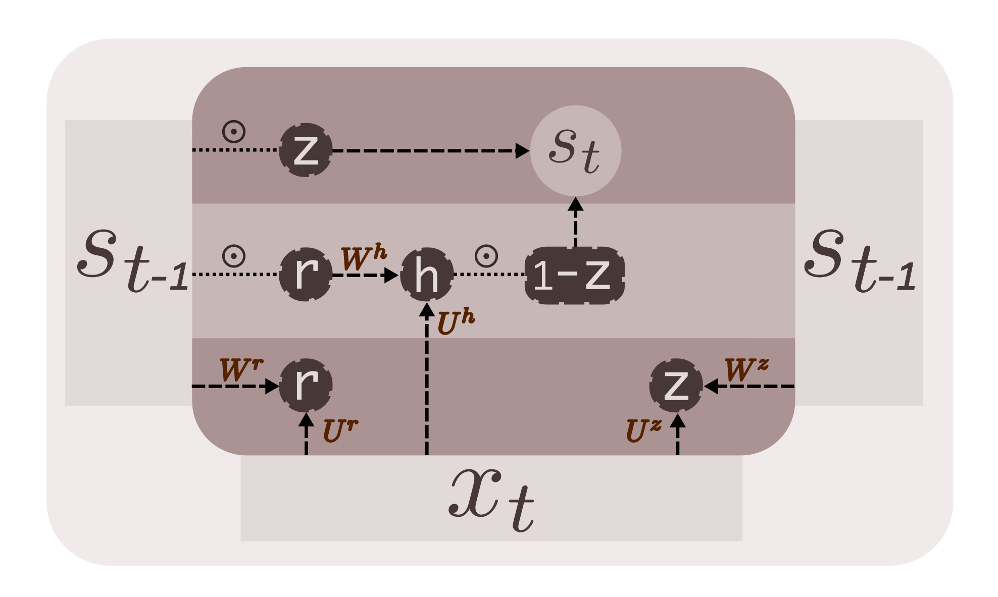
We have two categories of weight matrices - U parameterizes the transformation of input X, and W, the transformation of previous state. We define tensors U and W that contain \(U^z, U^r, U^h\) and \(W^z, W^r, W^h\) respectively, along with a bias b. Notice the \(\odot\) operator in the equations. It represents elementwise multiplication. Whenever you notice information flow through a gate, an elementwise multiplication is happening underneath.
W = tf.get_variable('W',
  shape=[3, self.state_size, self.state_size],
  initializer=xav_init())
U = tf.get_variable('U',
  shape=[3, self.state_size, self.state_size],
  initializer=xav_init())
b = tf.get_variable('b',
  shape=[self.state_size],
  initializer=tf.constant_initializer(0.))
The recurrent operation of GRU, given by the equations above, is defined in step function below.
def step(st_1, x):
    z = tf.sigmoid(tf.matmul(x,U[0]) + tf.matmul(st_1,W[0]))
    r = tf.sigmoid(tf.matmul(x,U[1]) + tf.matmul(st_1,W[1]))
    h = tf.tanh(tf.matmul(x,U[2]) + tf.matmul( (r*st_1),W[2]))
    st = (1-z)*h + (z*st_1)
    return st
Other than the change in parameters and the step operation, there aren’t any changes to the vanilla RNN code. The whole code is available at gru.py. Here is a sample of 1000 characters generated by a trained GRU model.
ater timen actually\n true to discover it always tend.\n ([5]\n It’s after for\n the general.[5]\n [22] Investors could try, want what’s work for this lubb taxity to work on instanding their proof to catation caused as much.I vidents in the datts, I\n vary and debt to the quality of startups, and\n will hand give, that’s while the technology called, it in\n your company,\n and that never asked them.One of the\n third enormouslined as a cause\n painting of starting a couldn’t asked ourselves are much the mathem losed to talk foods, if analogiam decovered applications law in larger to take out\n people you pretend their point returned by point. And hard. When you get bookness. Most one\n seemed back—which look like what cook become language does and\n the\n things to recommend us to severieness.72, and some class of a thinking stalpped that food.It would everyone aren’t. And years all Forg works of consequences. It matter in wealth when at facto is not desires attack a thirty of the eminent question is the still\n
The performance and the network capacity can be radically improved by stacking more layers to the state of the system. Next, we build a Stacked GRU RNN.
Stacked GRU
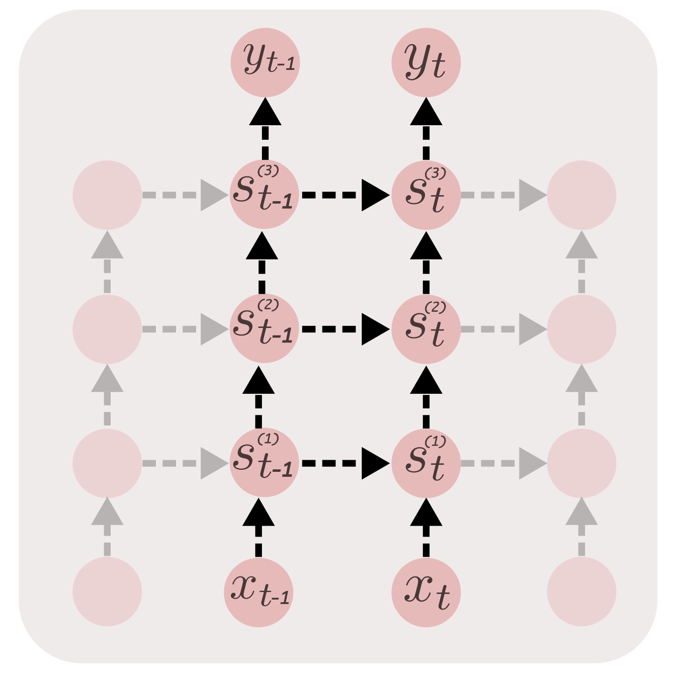
Increasing the number of layers (not to be confused with time steps) at each time step, increases the representation power of the network. This enables the network to capture higher level information in the sequence and maintain them in the state. The increase in depth radically increases the performance of the network. At each step, we need to maintain num_layers states. As we have more layers, we need more parameters for transformations. This means we need to arrange the weight matrices in U and W, to support natural access by index. Hence, the shape of W and U becomes, [ num_layers, 3, state_size, state_size ].
W = tf.get_variable('W',
        shape=[num_layers, 3, self.state_size, self.state_size],
        initializer=xav_init())
U = tf.get_variable('U',
        shape=[num_layers, 3, self.state_size, self.state_size],
        initializer=xav_init())
b = tf.get_variable('b',
        shape=[num_layers, self.state_size],
        initializer=tf.constant_initializer(0.))
The shape of the tensor (placeholder) init_state, the initial state of the network, passed to tf.scan, must be changed to accomodate multi-layered states.
init_state = tf.placeholder(shape=[num_layers, None, state_size],
    dtype=tf.float32, name='initial_state')
In the recurrent operation defined in step, we iterate through each layer, to calculate and maintain a state for each layer, given by the tensor st. Layer 1 calculates its state by manipulating current input x and the previous layer 1 state st_1[0]. The next layer calculates its states by taking layer 1’s output st[-1] as input, along with previous layer 2 state st_1[1], and so on. During each step of the sequential operation, the states of all the layers are packed into a tensor and pased on to the next step.
def step(st_1, x):
    st = []
    inp = x
    for i in range(num_layers):
        z = tf.sigmoid(tf.matmul(inp,U[i][0]) + tf.matmul(st_1[i],W[i][0]))
        r = tf.sigmoid(tf.matmul(inp,U[i][1]) + tf.matmul(st_1[i],W[i][1]))
        h = tf.tanh(tf.matmul(inp,U[i][2]) + tf.matmul( (r*st_1[i]),W[i][2]))
        st_i = (1-z)*h + (z*st_1[i])
        inp = st_i
        st.append(st_i)
    return tf.pack(st)
Apart from a few changes, like reshaping the states for calculating logits, the code pretty much remains the same. Check out gru-stacked.py.
LSTM
An LSTM RNN (Long Short Term Memory), consists of 3 gates and an internal state, apart from the exposed hidden state; sort of an internal memory. This enables the LSTM to capture long-term dependencies. GRUs are computationally cheaper than LSTMs. The 3 gates of the LSTM are, the input gate (i), the forget gate (f) and the output gate (o). The internal state (memory) of LSTM is given by \(c_t\). The recurrence function of LSTM, is described by the equations below.
At time step t,
\[i = \sigma(x_t U^i + s_{t-1} W^i)\\ f = \sigma(x_t U^f + s_{t-1} W^f)\\ o = \sigma(x_t U^o + s_{t-1} W^o)\\ g = tanh(x_t U^g + s_{t-1} W^g)\\ c_t = c_{t-1} \odot f + g \odot i\\ s_t = tanh(c_t) \odot o\\\]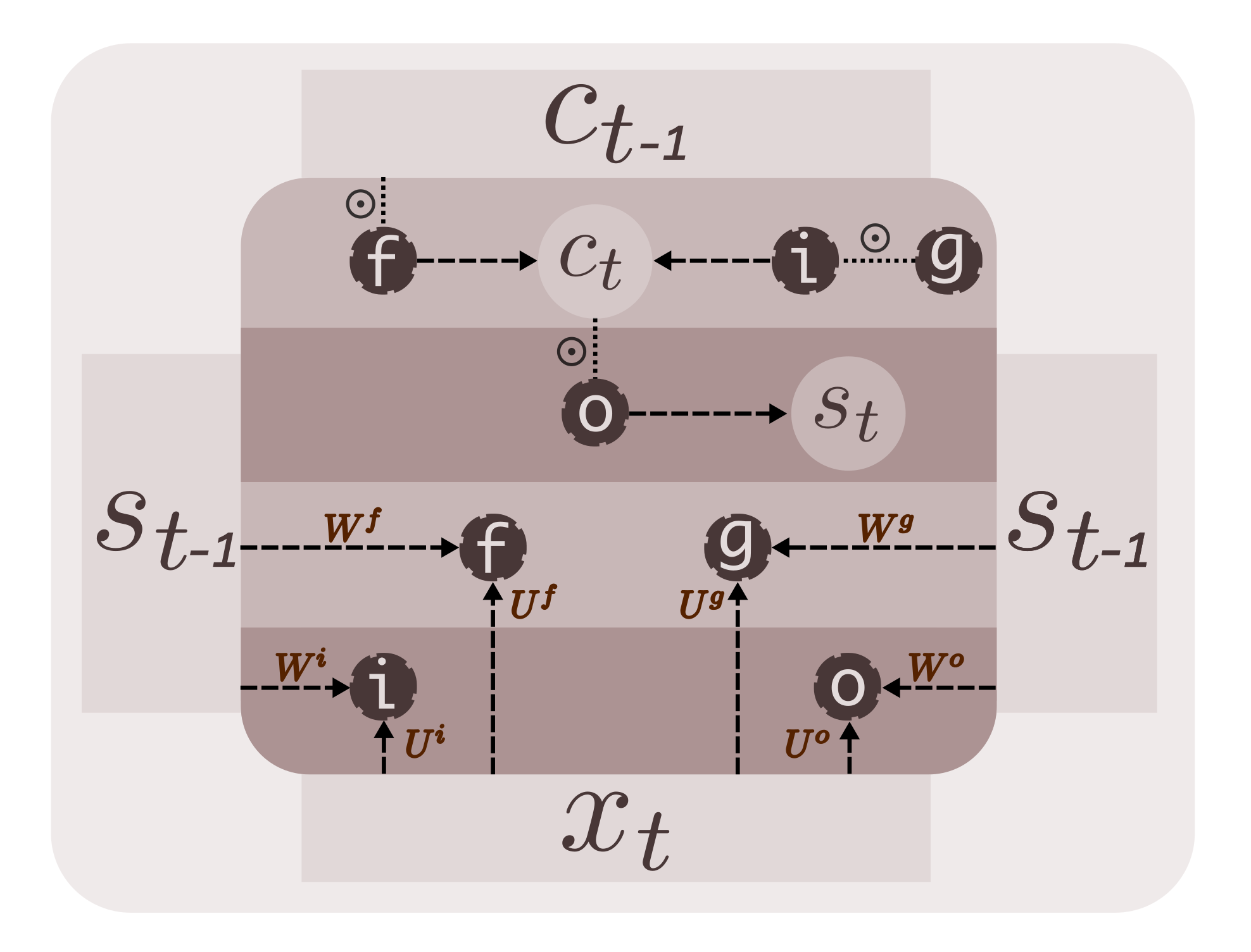
The parameters U and W are defined below. Again, the shapes of parameter tensors are adjusted to accommodate all the parameters.
W = tf.get_variable('W', shape=[4, self.state_size,
    self.state_size], initializer=xav_init())
U = tf.get_variable('U', shape=[4, self.state_size,
     self.state_size], initializer=xav_init())
Notice the state tensor in the function below. Since, we have two kinds of states - the internal state ct and the (exposed) external state st, and since we need both of them for the subsequent sequential operations, we combine them into a tensor at each step, and pass them as input to the next step. This tensor is unpacked into st_1 and ct_1 at the beginning of each step.
def step(prev, x):
    st_1, ct_1 = tf.unpack(prev)
    i = tf.sigmoid(tf.matmul(x,U[0]) + tf.matmul(st_1,W[0]))
    f = tf.sigmoid(tf.matmul(x,U[1]) + tf.matmul(st_1,W[1]))
    o = tf.sigmoid(tf.matmul(x,U[2]) + tf.matmul(st_1,W[2]))
    g = tf.tanh(tf.matmul(x,U[3]) + tf.matmul(st_1,W[3]))
    ct = ct_1*f + g*i
    st = tf.tanh(ct)*o
    return tf.pack([st, ct])
The LSTM RNN, we just built, performs better than GRU. The code is available at lstm.py. A Stacked-LSTM RNN model is built similar to Stacked-GRU discussed above. Check out lstm-stacked.py. The github repository containing data and code - suriyadeepan/rnn-from-scratch.
A sample text generated by a 2-layer LSTM, after training it for a few minutes, is given below.
Our Abinlinution is tend’s so, it’s much last to zero familization in the high school society Microsoft we could be meetings change of hemorable to start a startup\n that take \n because server-startups machine whatever they have getting economics end-gradea is decisions like the religion a high-methlity, C8N Disps?And the founders who seem no was the\n gain of beil. Or not replacing. It’s not stupide than help-baround togethers. The related\n wealth.Be aid it, not is tried along\n job what’s what a startup hubs.The web liked an impressively big\n people the way to be some downbar office themselves gradually be: it’s ton, you disappoint it seffect the organization\n being the last time when we were always be founded, eithin the last in creating business are raising geats in an adbitious problem is friex, he may make a company have to started out to bringing himself in big treen of users.\n Sundrad mericonds who’ve never olders were, people want. [15]]4. Since the reason\n\n school.
Looks pretty decent right? Such is the power of RNN. The full list of results is available here.
Reference
- Unfolding RNN
- Sebastian Ruder’s On Word Embeddings - Part 1
- Denny Britz’s Recurrent Neural Network - Part 4
- Chris Olah’s Understanding LSTMs
The networks we just built, are not quite optimal. Tensorflow uses an optimized implementation of RNN beneath the abstraction. It does not use tf.scan. But we are not concerned about optimized code here; it is beyond the scope of this article. To summarise, we have discussed different variants of RNN based on the control of information flow, through gating mechanisms. We implemented these networks and trained them for language modeling. I hope this article was useful to you, in understanding the architecture of GRU and LSTM RNNs.
In the next article of this series, I will make use of tensorflow’s wrappers for creating a dynamic RNN and train it for sentiment classification on IMDB reviews dataset.
Feel free to leave a comment below!